Data

The description of the methods, input data and results of the eGon-data pipeline is given in the following section. References to datasets and functions are integrated if more detailed information is required.

Main input data and their processing

All methods in the eGon-data workflow rely on public and freely available data from different external sources. The most important data sources and their processing within the eGon-data pipeline are described here.

Data bundle

The data bundle is published on zenodo. It contains several data sets, which serve as a basis for egon-data:

• Climate zones in Germany

• Data on eMobility individual trips of electric vehicles

• Spatial distribution of deep geothermal potentials in Germany

• Annual profiles in hourly resolution of electricity demand of private households

• Sample heat time series including hot water and space heating for single- and multi-familiy houses

• Hydrogen storage potentials in salt structures

• Information about industrial sites with DSM-potential in Germany

• Data extracted from the German grid development plan - power

• Parameters for the classification of gas pipelines

• Preliminary results from scenario generator pypsa-eur-sec

• German regions suitable to model dynamic line rating

• Eligible areas for wind turbines and ground-mounted PV systems

• Definitions of industrial and commercial branches

• Zensus data on households

• Geocoding of all unique combinations of ZIP code and municipality within the Marktstammdatenregister

For further description of the data including licenses and references please refer to the Zenodo repository.

Marktstammdatenregister

The Marktstammdatenregister (MaStR) is the register for the German electricity and gas market holding, among others, data on electricity and gas generation plants. In eGon-data it is used for status quo data on PV plants, wind turbines, biomass, hydro power plants, combustion power plants, nuclear power plants, geo- and solarthermal power plants, and storage units. The data are obtained from zenodo, where raw MaStR data, downloaded with the tool open-MaStR using the MaStR webservice, is provided. It contains all data from the MaStR, including possible duplicates. Currently, two versions are used:

• 2021-04-30

• 2022-11-17

The download is implemented in MastrData.

OpenStreetMap

OpenStreetMap (OSM) is a free, editable map of the whole world that is being built by volunteers and released with an open-content license. In eGon-data it is, among others, used to obtain information on land use as well as locations of buildings and amenities to spatially dissolve energy demand. The OSM data is downloaded from the Geofabrik download server, which holds extracts from the OpenStreetMap. Afterwards, they are imported to the database using osm2pgsql with a custom style file. The implementation of this can be found in OpenStreetMap.

In the OpenStreetMap dataset, the OSM data is filtered, processed and enriched with other data. This is described in the following subsections.

Amenity data

The data on amenities is used to disaggregate CTS demand data. It is filtered from the raw OSM data using tags listed in script osm_amenities_shops_preprocessing.sql, e.g. shops and restaurants. The filtered data is written to database table openstreetmap.osm_amenities_shops_filtered.

Building data

The data on buildings is required by several tasks in the pipeline, such as the disaggregation of household demand profiles or PV home systems to buildings, as well as the DIstribution Network Generat0r ding0 (see also Medium and low-voltage grids).

The data processing steps are:

• Extract buildings and filter using relevant tags, e.g. residential and commercial, see script osm_buildings_filter.sql for the full list of tags. Resulting tables:

  • All buildings: openstreetmap.osm_buildings

  • Filtered buildings: openstreetmap.osm_buildings_filtered

  • Residential buildings: openstreetmap.osm_buildings_residential

• Create a mapping table for building’s OSM IDs to the Zensus cells the building’s centroid is located in. Resulting tables:

  • boundaries.egon_map_zensus_buildings_filtered (filtered)

  • boundaries.egon_map_zensus_buildings_residential (residential only)

• Enrich each building by number of apartments from Zensus table society.egon_destatis_zensus_apartment_building_population_per_ha by splitting up the cell’s sum equally to the buildings. In some cases, a Zensus cell does not contain buildings but there is a building nearby which the no. of apartments is to be allocated to. To make sure apartments are allocated to at least one building, a radius of 77m is used to catch building geometries.

• Split filtered buildings into 3 datasets using the amenities’ locations: temporary tables are created in script osm_buildings_temp_tables.sql, the final tables in osm_buildings_amentities_results.sql. Resulting tables:

  • Buildings w/ amenities: openstreetmap.osm_buildings_with_amenities

  • Buildings w/o amenities: openstreetmap.osm_buildings_without_amenities

  • Amenities not allocated to buildings: openstreetmap.osm_amenities_not_in_buildings

As there are discrepancies between the Census data [Census] and OSM building data when both datasets are used to generate electricity demand profiles of households, synthetic buildings are added in Census cells with households but without buildings. This is done as part of the Demand_Building_Assignment dataset in function generate_synthetic_buildings. The synthetic building data are written to table openstreetmap.osm_buildings_synthetic. The same is done in case of CTS electricity demand profiles. Here, electricity demand is disaggregated to Census cells according to heat demand information from the Pan European Thermal Atlas [Peta]. In case there are Census cells with electricity demand assigned but no building or amenity data, synthetic buildings are added. This is done as part of the CtsDemandBuildings dataset in function create_synthetic_buildings. The synthetic building data are again written to table openstreetmap.osm_buildings_synthetic.

Street data

The data on streets is used in the DIstribution Network Generat0r ding0, e.g. for the routing of the grid. It is filtered from the raw OSM data using tags listed in script osm_ways_preprocessing.sql, e.g. highway=secondary. Additionally, each way is split into its line segments and their lengths is retained. The filtered streets data is written to database table openstreetmap.osm_ways_preprocessed and the filtered streets with segments to table openstreetmap.osm_ways_with_segments.

Grid models

Power grid models of different voltage levels form a central part of the eGon-data model, which is required for cross-grid-level optimization. In addition, sector coupling necessitates the representation of the gas grid infrastructure, which is also described in this section.

Electricity grid

High and extra-high voltage grids

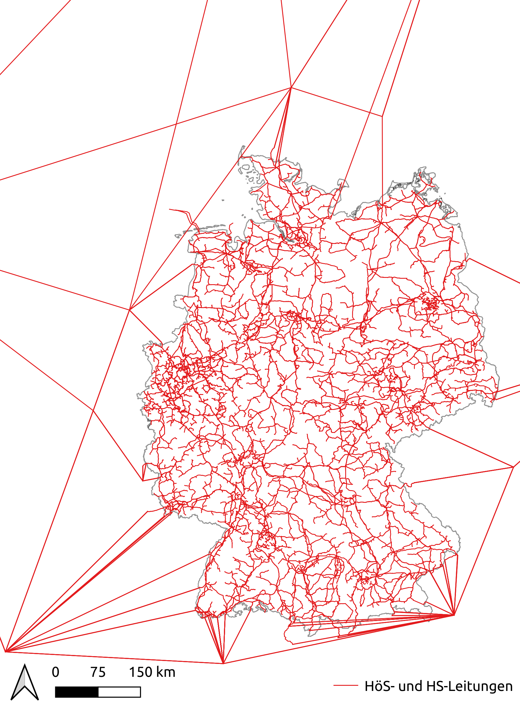
The model of the German extra-high (eHV) and high voltage (HV) grid is based on data retrieved from OpenStreetMap (OSM) (status January 2021) [OSM] and additional parameters for standard transmission lines from [Brakelmann2004]. To gather all required information, such as line topology, voltage level, substation locations, and electrical parameters, to create a calculable power system model, the *osmTGmod* tool was used. The corresponding dataset Osmtgmod executes osmTGmod and writes the resulting data to the database.

The resulting grid model includes the voltage levels 380, 220 and 110 kV and all substations interconnecting the different grid levels. Information about border crossing lines are as well extracted from OSM data by osmTGmod. For further information on the generation of the grid topology please refer to [Mueller2018]. The neighbouring countries are included in the model in a significantly lower spatial resolution with one or two nodes per country. The border crossing lines extracted by osmTGmod are extended to representative nodes of the respective country in dataset ElectricalNeighbours. The resulting grid topology is shown in the following figure.

Medium and low-voltage grids

Medium (MV) and low (LV) voltage grid topologies for entire Germany are generated using the python tool ding0 ding0. ding0 generates synthetic grid topologies based on high-resolution geodata and routing algorithms as well as typical network planning principles. The generation of the grid topologies is not part of eGon_data, but ding0 solely uses data generated with eGon_data, such as locations of HV/MV stations (see High and extra-high voltage grids), locations and peak demands of buildings in the grid (see Building data respectively Electricity), as well as locations of generators from MaStR (see Marktstammdatenregister). A full list of tables used in ding0 can be found in its config. An exemplary MV grid with one underlying LV grid is shown in figure Exemplary synthetic medium-voltage grid with underlying low-voltage grid generated with ding0. The grid data of all over 3.800 MV grids is published on zenodo.

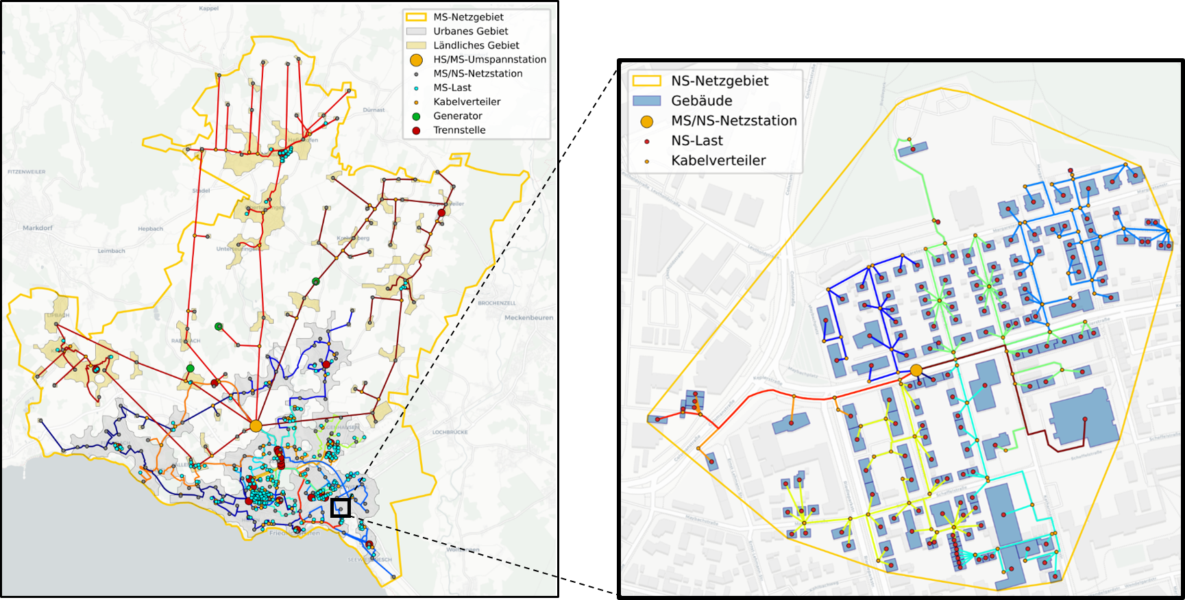
Exemplary synthetic medium-voltage grid with underlying low-voltage grid generated with ding0

Besides data on buildings and generators, ding0 requires data on the supplied areas by each grid. This is as well done in eGon_data and described in the following.

MV grid districts

Medium-voltage (MV) grid districts describe the area supplied by one MV grid. They are defined by one polygon that represents the supply area. Each MV grid district is connected to the HV grid via a single substation. An exemplary MV grid district is shown in figure Exemplary synthetic medium-voltage grid with underlying low-voltage grid generated with ding0 (orange line).

The MV grid districts are generated in the dataset MvGridDistricts. The methods used for identifying the MV grid districts are heavily inspired by Hülk et al. (2017) [Huelk2017] (section 2.3), but the implementation differs in detail. The main difference is that direct adjacency is preferred over proximity. For polygons of municipalities without a substation inside, it is iteratively checked for direct adjacent other polygons that have a substation inside. Speaking visually, a MV grid district grows around a polygon with a substation inside.

The grid districts are identified using three data sources

1. Polygons of municipalities (Vg250GemClean)

2. Locations of HV-MV substations (EgonHvmvSubstation)

3. HV-MV substation voronoi polygons (EgonHvmvSubstationVoronoi)

Fundamentally, it is assumed that grid districts (supply areas) often go along borders of administrative units, in particular along the borders of municipalities due to the concession levy. Furthermore, it is assumed that one grid district is supplied via a single substation and that locations of substations and grid districts are designed for aiming least lengths of grid line and cables.

With these assumptions, the three data sources from above are processed as follows:

• Find the number of substations inside each municipality

• Split municipalities with more than one substation inside

  • Cut polygons of municipalities with voronoi polygons of respective substations

  • Assign resulting municipality polygon fragments to nearest substation

• Assign municipalities without a single substation to nearest substation in the neighborhood

• Merge all municipality polygons and parts of municipality polygons to a single polygon grouped by the assigned substation

For finding the nearest substation, as already said, direct adjacency is preferred over closest distance. This means, the nearest substation does not necessarily have to be the closest substation in the sense of beeline distance. But it is the substation definitely located in a neighboring polygon. This prevents the algorithm to find solutions where a MV grid districts consists of multi-polygons with some space in between. Nevertheless, beeline distance still plays an important role, as the algorithm acts in two steps

1. Iteratively look for neighboring polygons until there are no further polygons

2. Find a polygon to assign to by minimum beeline distance

The second step is required in order to cover edge cases, such as islands.

For understanding how this is implemented into separate functions, please see define_mv_grid_districts.

Load areas

Load areas (LAs) are defined as geographic clusters where electricity is consumed. They are used in ding0 to determine the extent and number of LV grids. Thus, within each LA there are one or multiple MV-LV substations, each supplying one LV grid. Exemplary load areas are shown in figure Exemplary synthetic medium-voltage grid with underlying low-voltage grid generated with ding0 (grey and orange areas).

The load areas are set up in the LoadArea dataset. The methods used for identifying the load areas are heavily inspired by Hülk et al. (2017) [Huelk2017] (section 2.4).

Gas grid

In the gas sector, only the transport grids are represented. They are modelled with bidirectional PyPSA links which allow to represent the energy exchange between distinct PyPSA buses. No losses are considered and the energy that can be transferred through a pipeline is limited by the e_nom parameter.

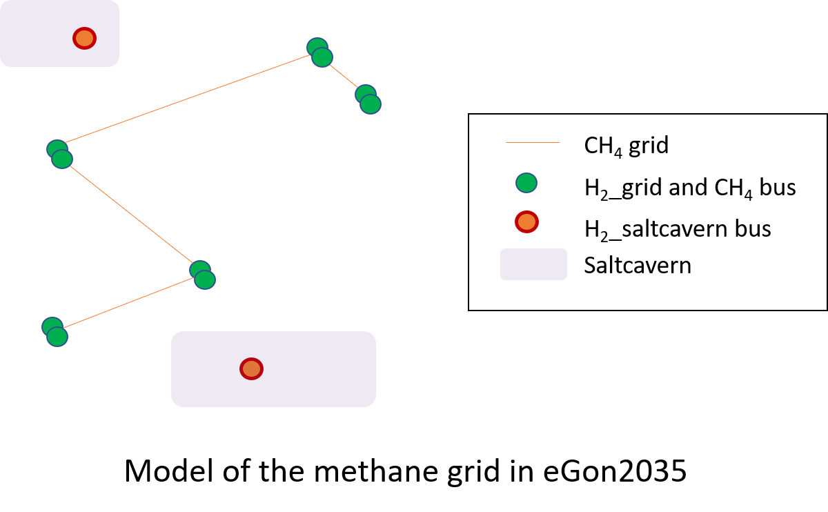
In the scenario eGon2035, only the methane grid is modelled.

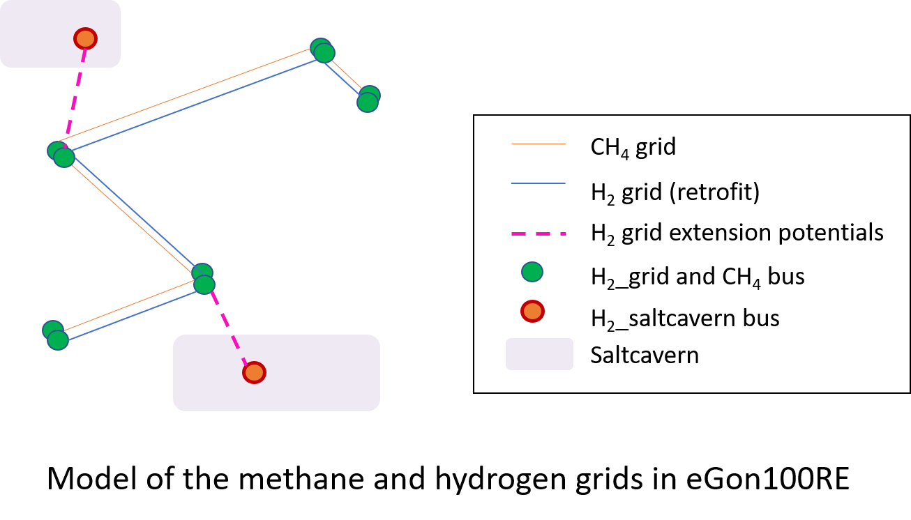
In the scenario eGon100RE, there are tree type of gas grid:

• the remaining methane grid,

• the retrofitted hydrogen grid,

• the potential hydrogen grid extension (only present in Germany).

To determine the topology of the grid, the status quo methane grid is used, with the data from SciGRID_gas [SciGRID_gas].

In the scenario eGon2035, the capacities of the methane pipelines are determined using the status quo pipeline diameters [SciGRID_gas] and the correspondence table [Kunz]. These capacities are fixed.

There are two types of hydrogen buses and none of them are connected through a grid:

• H2_grid buses: these buses are located at the places than the methane buses,

• H2_saltcavern buses: these buses are located at the intersection of power substations and potential saltcavern areas, adapted for hydrogen storage.

In this scenario, there are no hydrogen bus modelled in the neighboring countries.

The modelling of the methane grid in the scenario eGon2035 is represented below.

The implementation of these data is detailed respectively in the gas_grid and hydrogen_etrago.bus pages of our documentation.

In the scenario eGon100RE, the methane grid has the same topology than in the scenario eGon2035. The capacities of the methane pipelines are still fixed, but they are reduced, because a part of the grid is retrofitted into an hydrogen grid.

The retrofitted hydrogen grid has the same topology than the methane grid. The share of the methane grid which is retrofitted is calculated by the PyPSA-eur-sec run.

The potential hydrogen grid extensions link each hydrogen saltcavern to its nearest (retrofitted) hydrogen grid bus. The extension has no upper boundary and its technical parameters are taken from the PyPSA technology data [technoData]. This option is modelled exclusively in Germany.

The modelling of the methane grid in the scenario eGon100RE is represented below.

The implementation of these data is detailed respectively in the gas_grid and h2_grid pages of our documentation.

The cross-bordering pipelines capacities are taken respectively from the TYNDP [TYNDP] for eGon2035 and from PyPSA-eur-sec for eGon100RE.

For the cross-bordering gas pipelines with Germany, the capacity is uniformly distributed between the all pipelines connecting one country to Germany.

The implementation of these data is detailed respectively in the gas_neighbours.eGon2035.grid and insert_gas_neigbours_eGon100RE pages of our documentation.

Demand

Electricity, heat and gas demands from different consumption sectors are taken into account in eGon-data. The related methods to distribute and process the demand data are described in the following chapters for the different consumption sectors separately.

Electricity

The electricity demand considered includes demand from the residential, commercial and industrial sector. The target values for scenario eGon2035 are taken from the German grid development plan from 2021 [NEP2021], whereas the distribution on NUTS3-levels corresponds to the data from the research project DemandRegio [demandregio]. The following table lists the electricity demands per sector:

Electricity demand per sector

Sector	Annual electricity demand in TWh
residential	115.1
commercial	123.5
industrial	259.5

A further spatial and temporal distribution of the electricity demand is needed for the subsequent grid optimization. Therefore different sector-specific distributions methods were developed and applied.

Residential electricity demand

The annual electricity demands of households on NUTS3-level from DemandRegio are scaled to meet the national target values for the respective scenario in dataset DemandRegio. A further spatial and temporal distribution of residential electricity demands is performed in HouseholdElectricityDemand as described in [Buettner2022].

The allocation of the chosen electricity profiles in each census cell to buildings is conducted in the dataset Demand_Building_Assignment. For each cell, the profiles are randomly assigned to an OSM building within this cell. If there are more profiles than buildings, all additional profiles are further randomly allocated to buildings within the cell. Therefore, multiple profiles can be assigned to one building, making it a multi-household building. In case there are no OSM buildings that profiles can be assigned to, synthetic buildings are generated with a dimension of 5m x 5m. The number of synthetically created buildings per census cell is determined using the Germany-wide average of profiles per building (value is rounded up and only census cells with buildings are considered). The profile ID each building is assigned is written to data base table demand.egon_household_electricity_profile_of_buildings. Synthetically created buildings are written to data base table openstreetmap.osm_buildings_synthetic. The household electricity peak load per building is written to database table demand.egon_building_electricity_peak_loads. Drawbacks and limitations of the allocation to specific buildings are discussed in the dataset docstring of Demand_Building_Assignment.

The result is a consistent dataset across aggregation levels with an hourly resolution.

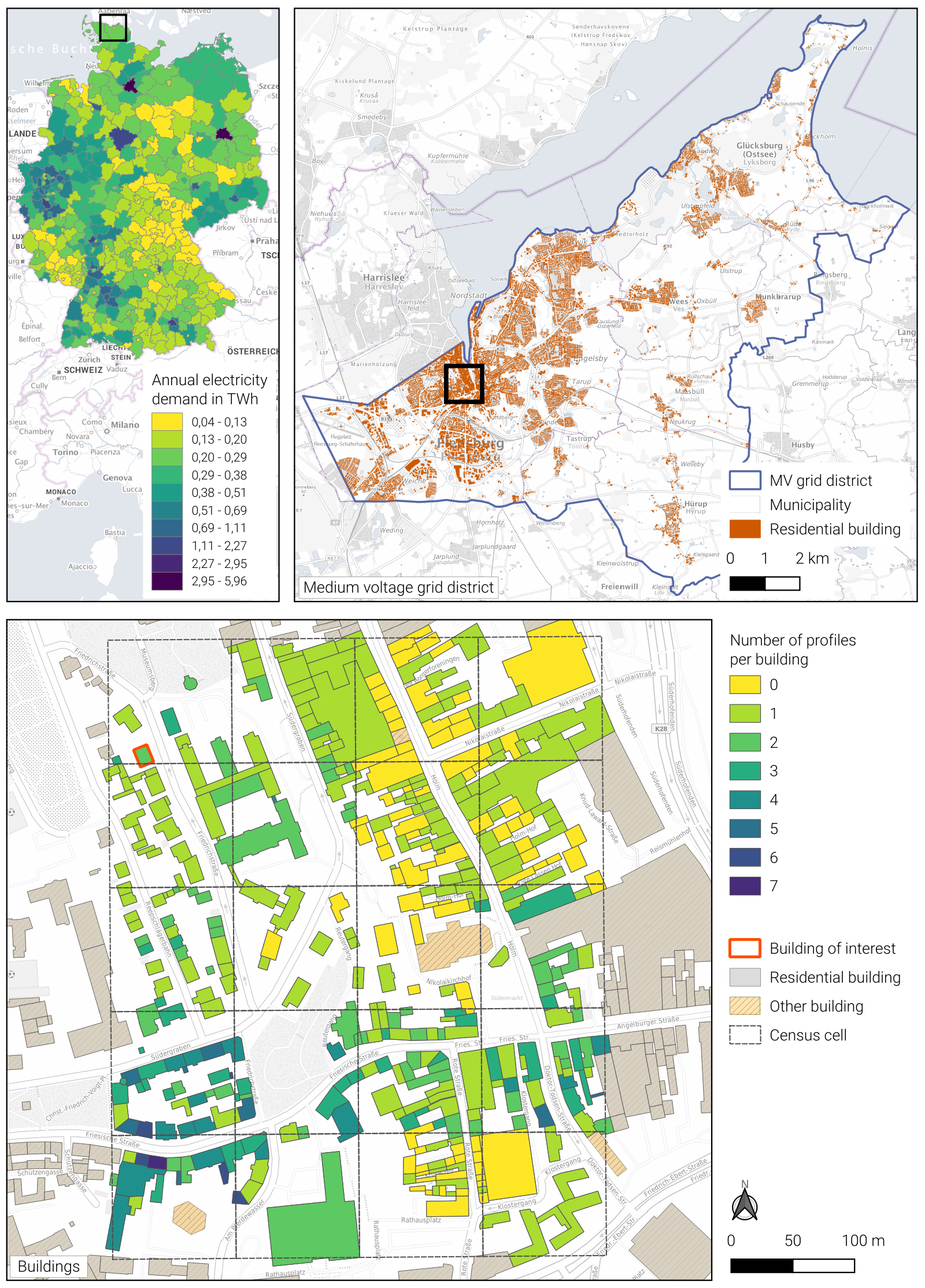
Electricity demand on NUTS 3-level (upper left); Exemplary MVGD (upper right); Study region in Flensburg (20 Census cells, bottom) from [Buettner2022]

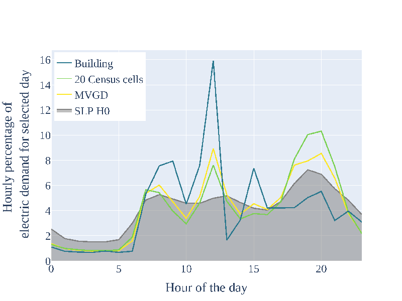
Electricity demand time series on different aggregation levels from [Buettner2022]

Commercial electricity demand

The distribution of electricity demand from the commercial, trade and service (CTS) sector is also based on data from DemandRegio, which provides annual electricity demands on NUTS3-level for Germany. In dataset CtsElectricityDemand the annual electricity demands are further distributed to census cells (100x100m cells from [Census]) based on the distribution of heat demands, which is taken from the Pan-European Thermal Atlas (PETA) version 5.0.1 [Peta]. For further information refer to section Heat.

Spatial disaggregation of CTS demand to buildings

The spatial disaggregation of the annual CTS demand to buildings is conducted in the dataset CtsDemandBuildings. Both the electricity demand as well as the heat demand is disaggregated in the dataset. Here, only the disaggregation of the electricity demand is described. The disaggregation of the heat demand is analogous to it. More information on the resulting tables is given in section Heat.

The workflow generally consists of three steps. First, the annual demand from Peta5 [Peta] is used to identify census cells with demand. Second, Openstreetmap [OSM] data on buildings and amenities is used to map the demand to single buildings. If no sufficient OSM data are available, new synthetic buildings and if necessary synthetic amenities are generated. Third, each building’s share of the HV-MV substation demand profile is determined based on the number of amenities within the building and the census cell(s) it is in.

The workflow is in more detail shown in figure Workflow for the disaggregation of the annual CTS demand to buildings and described in the following.

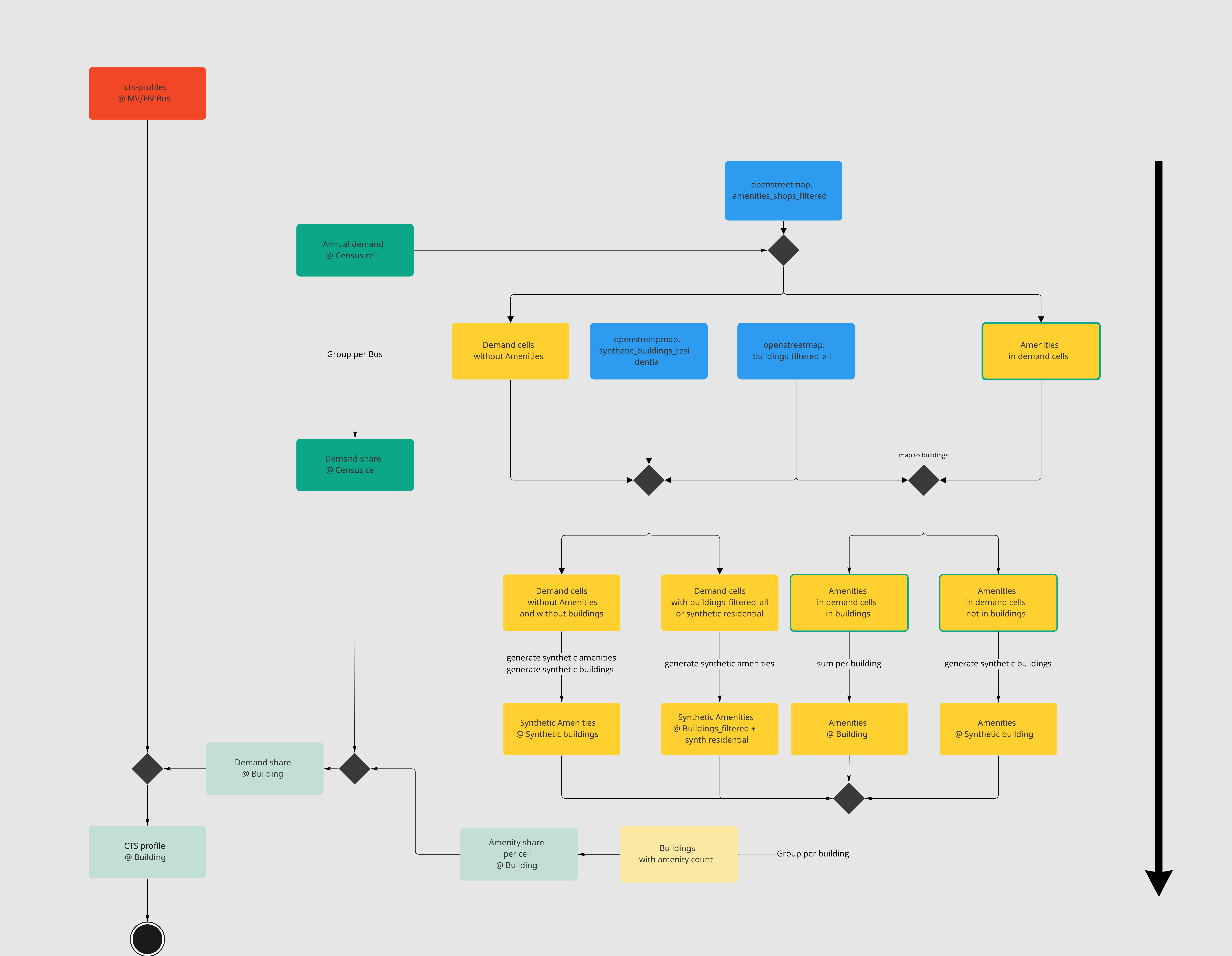
Workflow for the disaggregation of the annual CTS demand to buildings

In the OpenStreetMap dataset, we filtered all OSM buildings and amenities for tags we relate to the CTS sector. Amenities are mapped to intersecting buildings and then intersected with the annual demand at census cell level. We obtain census cells with demand that have amenities within and census cells with demand that don’t have amenities within. If there is no data on amenities, synthetic ones are assigned to existing buildings. We use the median value of amenities per census cell in the respective MV grid district to determine the number of synthetic amenities. If no building data is available, a synthetic building with a dimension of 5m x 5m is randomly generated. This also happens for amenities that couldn’t be assigned to any OSM building. We obtain four different categories of buildings with amenities:

• Buildings with amenities

• Synthetic buildings with amenities

• Buildings with synthetic amenities

• Synthetic buildings with synthetic amenities

Synthetically created buildings are written to data base table openstreetmap.osm_buildings_synthetic. Information on the number of amenities within each building with CTS, comprising OSM buildings and synthetic buildings, is written to database table openstreetmap.egon_cts_buildings.

To determine each building’s share of the HV-MV substation demand profile, first, the share of each building on the demand per census cell is calculated using the number of amenities per building. Then, the share of each census cell on the demand per HV-MV substation is determined using the annual demand defined by Peta5. Both shares are finally multiplied and summed per building ID to determine each building’s share of the HV-MV substation demand profile. The summing per building ID is necessary, as buildings can lie in multiple census cells and are therefore assigned a share in each of these census cells. The share of each CTS building on the CTS electricity demand profile per HV-MV substation in each scenario is saved to the database table demand.egon_cts_electricity_demand_building_share. The CTS electricity peak load per building is written to database table demand.egon_building_electricity_peak_loads.

Drawbacks and limitations as well as assumptions and challenges of the disaggregation are discussed in the dataset docstring of CtsDemandBuildings.

Industrial electricity demand

To distribute the annual industrial electricity demand OSM landuse data as well as information on industrial sites are taken into account. In a first step (CtsElectricityDemand) different sources providing information about specific sites and further information on the industry sector in which the respective industrial site operates are combined. Here, the three data sources [Hotmaps], [sEEnergies] and [Schmidt2018] are aligned and joined. Based on the resulting list of industrial sites in Germany and information on industrial landuse areas from OSM [OSM] which where extracted and processed in OsmLanduse the annual demands were distributed. The spatial and temporal distribution is performed in IndustrialDemandCurves. For the spatial distribution of annual electricity demands from DemandRegio [demandregio] which are available on NUTS3-level are in a first step evenly split 50/50 between industrial sites and OSM-polygons tagged as industrial areas. Per NUTS-3 area the respective shares are then distributed linearily based on the area of the corresponding landuse polygons and evenly to the identified industrial sites. In a next step the temporal disaggregation of the annual demands is carried out taking information about the industrial sectors and sector-specific standard load profiles from [demandregio] into account. Based on the resulting time series and their peak loads the corresponding grid level and grid connections point is identified.

Electricity demand in neighbouring countries

The neighbouring countries considered in the model are represented in a lower spatial resolution of one or two buses per country. The national demand timeseries in an hourly resolution of the respective countries is taken from the Ten-Year Network Development Plan, Version 2020 [TYNDP]. In case no data for the target year is available the data is is interpolated linearly. Refer to the corresponding dataset for detailed information: ElectricalNeighbours.

Heat

Heat demands comprise space heating and drinking hot water demands from residential and commercial trade and service (CTS) buildings. Process heat demands from the industry are, depending on the required temperature level, modelled as electricity, hydrogen or methane demand.

The spatial distribution of annual heat demands is taken from the Pan-European Thermal Atlas version 5.0.1 [Peta]. This source provides data on annual European residential and CTS heat demands per census cell for the year 2015. In order to model future demands, the demand distribution extracted by Peta is then scaled to meet a national annual demand from external sources. The following national demands are taken for the selected scenarios:

Heat demands per sector and scenario

	Residential sector	CTS sector	Sources
eGon2035	379 TWh	122 TWh	[Energiereferenzprognose]
eGon100RE	284 TWh	89 TWh	[Energiereferenzprognose]

The resulting annual heat demand data per census cell is stored in the database table demand.egon_peta_heat. The implementation of these data processing steps can be found in HeatDemandImport.

Figure Spatial distribution of residential heat demand per census cell in scenario eGon2035 shows the census cell distribution of residential heat demands for scenario eGon2035, categorized for different levels of annual demands.

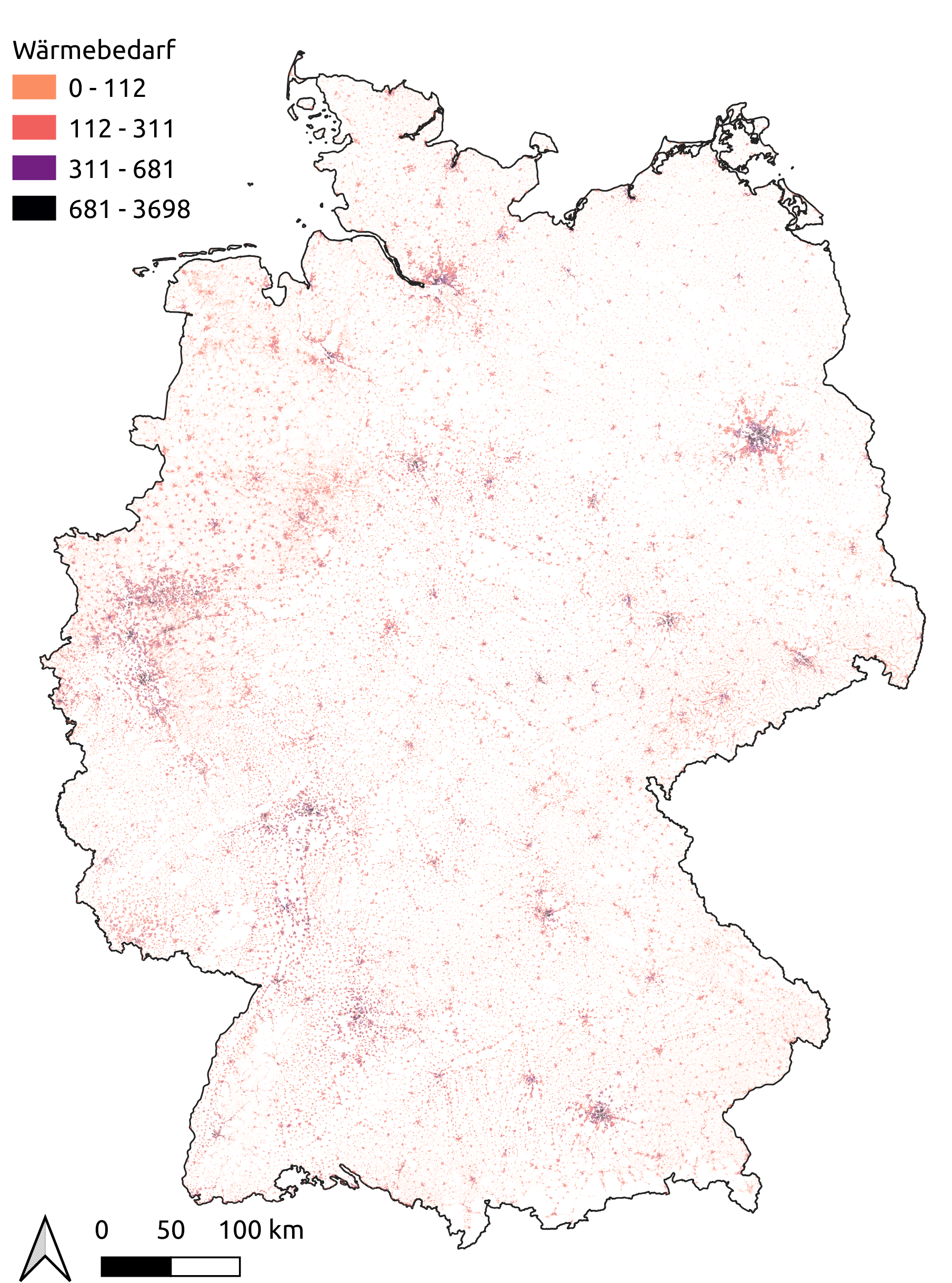
Spatial distribution of residential heat demand per census cell in scenario eGon2035

In a next step, the annual demand per census cell is further disaggregated to buildings. In case of residential buildings the demand is equally distributed to all residential buildings within the census cell. The annual demand per residential building is not saved in any database table but needs to be calculated from the annual demand in the census cell in table demand.egon_peta_heat and the number of residential buildings in table demand.egon_heat_timeseries_selected_profiles (see also query below). The disaggregation of the annual CTS heat demand per census cell to buildings is done analogous to the disaggregation of the electricity demand, which is in detail described in section Spatial disaggregation of CTS demand to buildings. The share of each CTS building of the corresponding HV-MV substation’s heat profile is for both the eGon2035 and eGon100RE scenario written to the database table EgonCtsHeatDemandBuildingShare. The peak heat demand per building, including residential and CTS demand, in the two scenarios eGon2035 and eGon100RE is calculated in the datasets HeatPumps2035 and HeatPumpsPypsaEurSec, respectively, and written to table demand.egon_building_heat_peak_loads.

The hourly heat demand profiles are for both sectors created in the Dataset HeatTimeSeries. For residential heat demand profiles a pool of synthetically created bottom-up demand profiles is used. Depending on the mean temperature per day, these profiles are randomly assigned to each residential building. The methodology is described in detail in [Buettner2022]. Data on residential heat demand profiles is stored in the database within the tables demand.egon_heat_timeseries_selected_profiles, demand.egon_daily_heat_demand_per_climate_zone, boundaries.egon_map_zensus_climate_zones. To create the profiles for a selected building, these tables have to be combined, e.g. like this:

SELECT (b.demand/f.count * UNNEST(e.idp) * d.daily_demand_share)*1000 AS demand_profile
FROM (SELECT * FROM demand.egon_heat_timeseries_selected_profiles,
UNNEST(selected_idp_profiles) WITH ORDINALITY as selected_idp) a
JOIN demand.egon_peta_heat b
ON b.zensus_population_id = a.zensus_population_id
JOIN boundaries.egon_map_zensus_climate_zones c
ON c.zensus_population_id = a.zensus_population_id
JOIN demand.egon_daily_heat_demand_per_climate_zone d
ON (c.climate_zone = d.climate_zone AND d.day_of_year = ordinality)
JOIN demand.egon_heat_idp_pool e
ON selected_idp = e.index
JOIN (SELECT zensus_population_id, COUNT(building_id)
FROM demand.egon_heat_timeseries_selected_profiles
GROUP BY zensus_population_id
) f
ON f.zensus_population_id = a.zensus_population_id
WHERE a.building_id = SELECTED_BUILDING_ID
AND b.scenario = 'eGon2035'
AND b.sector = 'residential';

Exemplary resulting residential heat demand time series for a selected day in winter and summer considering different aggregation levels are visualized in figures Temporal distribution of residential heat demand for a selected day in winter and Temporal distribution of residential heat demand for a selected day in summer.

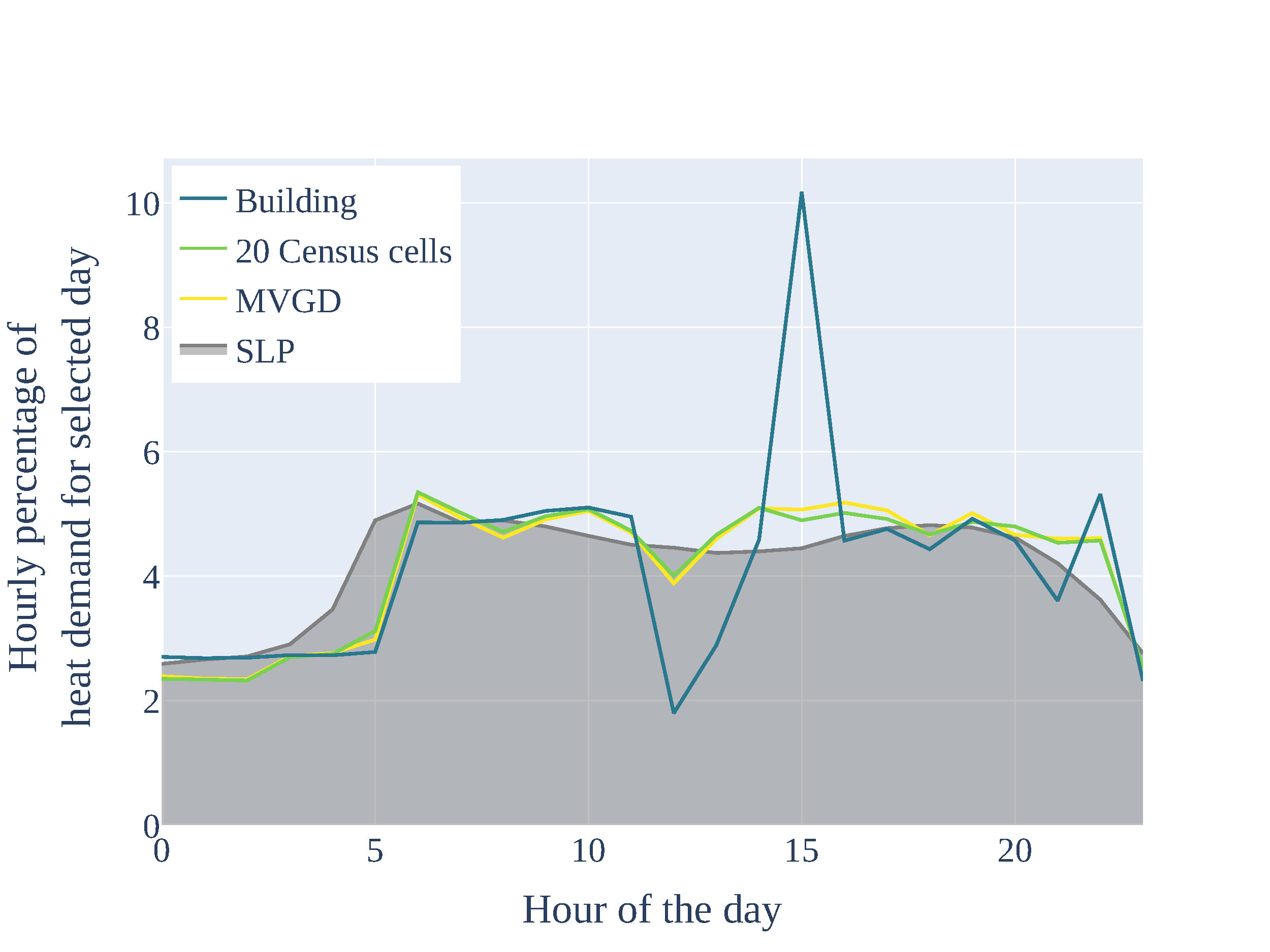
Temporal distribution of residential heat demand for a selected day in winter

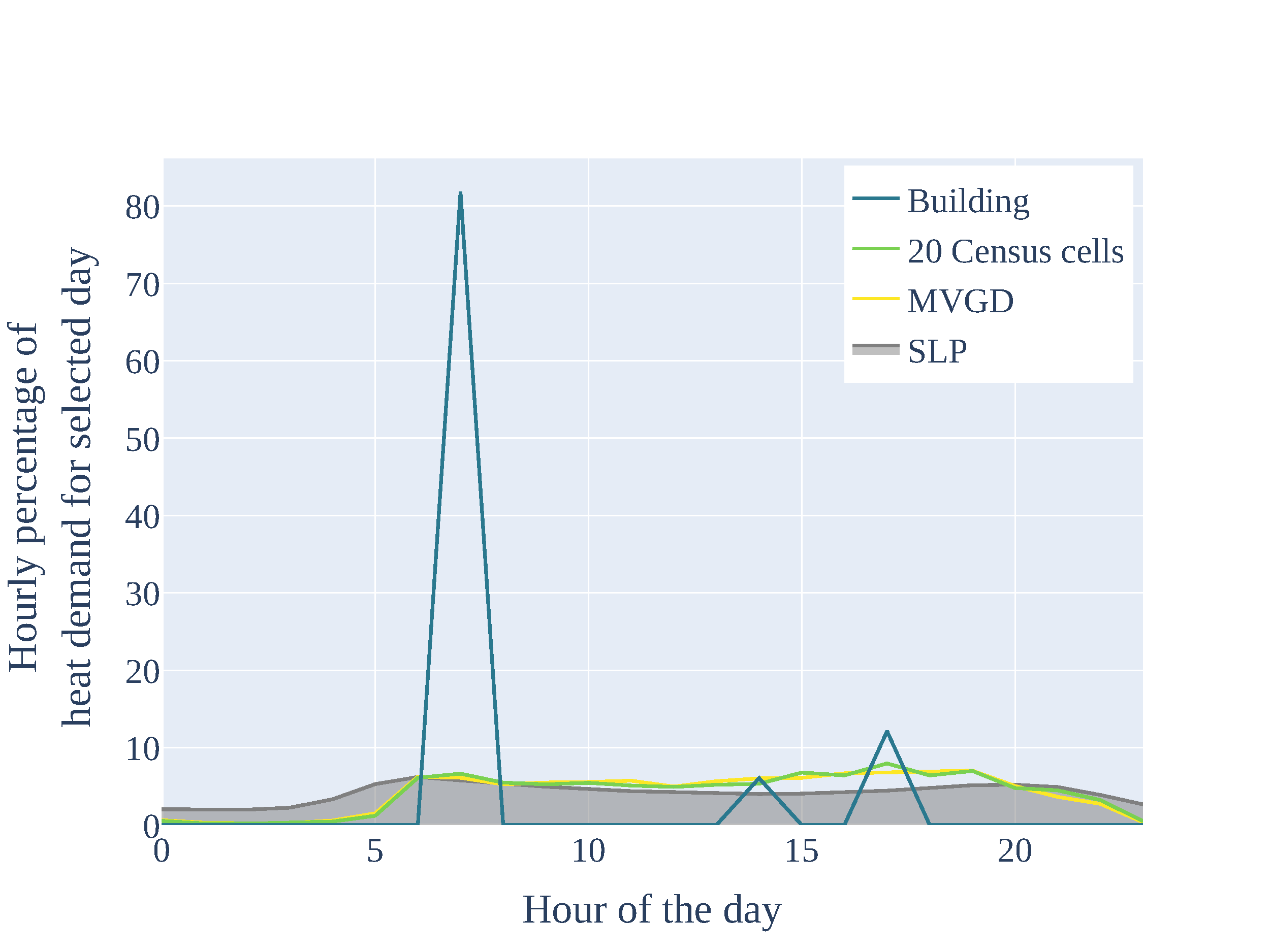
Temporal distribution of residential heat demand for a selected day in summer

The temporal disaggregation of CTS heat demand is done using Standard Load Profiles Gas from demandregio [demandregio] considering different profiles per CTS branch.

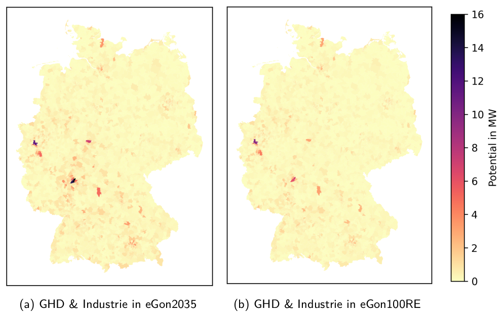
Gas

The industrial gas demand is modelled with PyPSA loads.

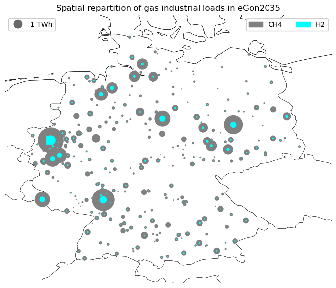
In the scenario eGon2035, the industrial gas loads in Germany are taken directly from the eXtremos project data [eXtremos]. They model the hourly-resolved industrial loads in Germany with a NUTS-3 spatial resolution, for methane (\(CH_4\)), as well as for hydrogen (\(H_2\)), for the year 2035.

The spatial repartition of these loads is represented in the figure below (methane demand in grey and hydrogen in cyan). The size of the rounds on the figure corresponds to the total annual demand at the considered spot in the scenario eGon2035.

In eGon100RE, the global industrial demand for methane and hydrogen (for whole Germany and for one year) is calculated by the PyPSA-eur-sec run. The spatial and the temporal repartitions used to distribute these values are corresponding to the spatial and temporal repartition of the hydrogen industrial demand from the eXtremos project [eXtremos] for the year 2050. (The same repartition is used, due to the lack of data were available for methane, because the eXtremos project considers that there won’t be any industrial methane load in 2050.)

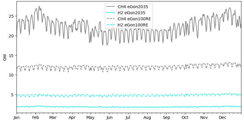
The figure above shows the temporal evolution of the methane (in grey) and hydrogen (in cyan) industrial demands in the year for both scenarios (eGon100RE in dashed). The total demands for whole Germany are to be found in the following table.

Total indutrial hydrogen and methane demands in Germany considered in eGon-data

	eGon2035	eGon100RE
\(CH_4\) (in TWh)	195	105
\(H_2\) (in TWh)	16	42

The hydrogen loads are attributed only to the H2_grid buses.

The implementation of these data is detailed in the industrial_gas_demand page of our documentation.

In the scenario eGon2035, there are no hydrogen buses modelled in the neighboring countries. For this reason, the hydrogen industrial demand is there attributed to the electrical sector. The total demand is taken from the ‘Distributed Energy’ scenario of the Ten-Year Network Development Plan 2020 ([TYNDP]). For the year 2035, it has been linearly interpolated between the values for the year 2030 and 2040. These industrial hydrogen loads are considered as constant in time. In other words, at each hour of the year, the same load should by fulfilled by electricity to supply the hydrogen industrial demand.

Contrary to all the other loads described in the section, the modelled methane load abroad includes not only the industrial demand, but also the heat demand, that is supplied by methane. The total demand is again taken from the ‘Distributed Energy’ scenario of the TYNDP 2020 (linear interpolation between 2030 and 2040). For the temporal disaggregation of the demand in the year, the time series ‘rural heat’ from PyPSA-eur-sec is used to approximated the temporal profile, because the heat sector represents the biggest load.

The implementation of these data is detailed in the gas_neighbours.eGon2035 page of our documentation.

In the scenario eGon100RE, the industrial gas loads (for methane as well as for hydrogen) in the neighboring countries are directly imported from the PyPSA-eur-sec run.

Mobility

Motorized individual travel

The electricity demand data of motorized individual travel (MIT) for both the eGon2035 and eGon100RE scenario is set up in the MotorizedIndividualTravel dataset. For the eGon2035, the workflow is visualised in figure Workflow to set up charging demand data for MIT in the eGon2035 scenario. The workflow for the eGon100RE scenario is analogous to the workflow for the eGon2035 scenario. In a first step, pre-generated SimBEV trip data, including information on driving, parking and (user-oriented) charging times is downloaded. In the second step, the number of EVs in each MV grid district in the future scenarios is determined. Last, based on the trip data and the EV numbers, charging time series as well as time series to model the flexibility of EVs are set up. In the following, these steps are explained in more detail.

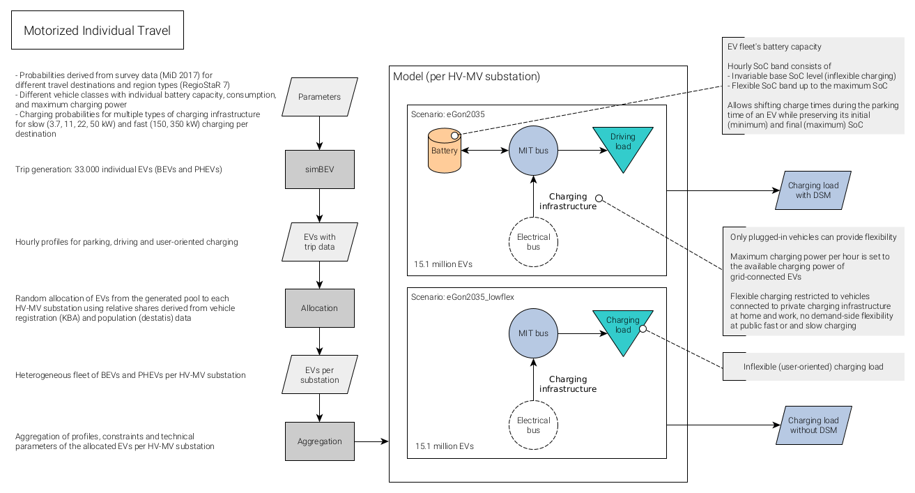
Workflow to set up charging demand data for MIT in the eGon2035 scenario

The trip data are generated using a modified version of SimBEV v0.1.3. SimBEV generates driving and parking profiles for battery electric vehicles (BEVs) and plug-in hybrid electric vehicles (PHEVs) based on MID survey data [MiD2017] per RegioStaR7 region type [RegioStaR7_2020]. The data contain information on energy consumption during the drive, as well as on the availability of charging points at the parking location and in case of an available charging point the corresponding charging demand, charging power and charging point use case (home charging point, workplace charging point, public charging point and fast charging point). Different vehicle classes are taken into account whose assumed technical data is given in table Differentiated EV types and corresponding technical data. Moreover, charging probabilities for multiple types of charging infrastructure are presumed based on [NOW2020] and [Helfenbein2021]. Given these assumptions, trip data for a pool of 33.000 EV-types is pre-generated and provided through the data bundle (see Data bundle). The data is as well written to database tables EgonEvTrip, containing information on the driving and parking times of each EV, and EgonEvPool, containing information on the type of EV and RegioStaR7 region the trip data corresponds to. The complete technical data and assumptions of the SimBEV run can be found in the metadata_simbev_run.json file, that is provided along with the trip data through the data bundle. The metadata is as well written to the database table EgonEvMetadata.

Differentiated EV types and corresponding technical data

Technology	Size	Max. slow charging capacity in kW	Max. fast charging capacity in kW	Battery capacity in kWh	Energy consumption in kWh/km
BEV	mini	11	120	60	0.1397
BEV	medium	22	350	90	0.1746
BEV	luxury	50	350	110	0.2096
PHEV	mini	3.7	40	14	0.1425
PHEV	medium	11	40	20	0.1782
PHEV	luxury	11	120	30	0.2138

The assumed total number of EVs in Germany is 15.1 million in the eGon2035 scenario (according to the network development plan [NEP2021] (Scenario C 2035)) and 25 million in the eGon100RE scenario (own assumption). To spatially disaggregate the charging demand, the total number of EVs per EV type is first allocated to MV grid districts based on vehicle registration [KBA] and population [Census] data (see function allocate_evs_numbers). The resulting number of EVs per EV type in each MV grid district in each scenario is written to the database table EgonEvCountMvGridDistrict. Each MV grid district is then assigned a random pool of EV profiles from the pre-generated trip data based on the RegioStaR7 region [RegioStaR7_2020] the grid district is assigned to and the counts per EV type (see function allocate_evs_to_grid_districts). The results are written to table EgonEvMvGridDistrict.

On the basis of the assigned EVs per MV grid district and the trip data, charging demand time series in each MV grid district can be determined. For inflexible charging (see lower right in figure Workflow to set up charging demand data for MIT in the eGon2035 scenario) it is assumed that the EVs are charged with full power as soon as they arrive at a charging station until they are fully charged. The respective charging power and demand is obtained from the trip data. The individual charging demand time series per EV are summed up to obtain the charging time series per MV grid district. The generation of time series to model flexible charging of EVs (upper right in figure Workflow to set up charging demand data for MIT in the eGon2035 scenario) is described in section Flexible charging of EVs.

For grid analyses of the MV and LV level, the charging demand needs to be further disaggregated within the MV grid districts. To this end, potential charging sites are determined. These potential charging sites are then used to allocate the charging demand of the EVs in each MV grid district to specific charging points. This allocation is not done in eGon-data but in the eDisGo tool and further described in the eDisGo documentation.

The determination of potential charging sites is conducted in class MITChargingInfrastructure. The results are written to database table EgonEmobChargingInfrastructure. The approach used to determine potential charging sites is based on the method implemented in TracBEV. Four use cases for charging points are differentiated - home, work, public and high-power charging (hpc). The potential charging sites are determined based on geographical data. Each possible charging site is assigned an attractivity that represents the likelihood that a charging point is installed at that site. The used approach is for each use case shortly described in the following:

• Home charging: The allocation of home charging stations is based on the number of apartments in each 100 x 100 m grid given by the Census 2011 [Census]. The cell with the highest number of apartments receives the highest attractivity.

• Work charging: The allocation of work charging stations is based on the area classification obtained from OpenStreetMap [OSM] using the landuse key. Work charging stations are allocated to areas tagged with commercial, retail or industrial. The attractivity of each area depends on the size of the area as well as the classification. Commercial areas receive the highest attractivity, followed by retail areas. Industrial areas are ranked lowest.

• Public charging (slow): The basis for the allocation of public charging stations are points of interest (POI) from OSM [OSM]. POI can be schools, shopping malls, supermarkets, etc. The attractivity of each POI is determined by empirical studies conducted in previous projects.

• High-power charging: The basis for the allocation of fast charging stations are the locations of existing petrol stations obtained from OSM [OSM]. The locations are ranked randomly at the moment.

The necessary input data is downloaded from zenodo.

Heavy-duty transport

In the context of the eGon project, it is assumed that all e-trucks will be completely hydrogen-powered. The hydrogen demand data of all e-trucks is set up in the HeavyDutyTransport dataset for both the eGon2035 and eGon100RE scenario.

In both scenarios the hydrogen consumption is assumed to be 6.68 kgH2 per 100 km with an additional supply chain leakage rate of 0.5 % (see here).

For the eGon2035 scenario the ramp-up figures are taken from the network development plan [NEP2021] (Scenario C 2035). According to this, 100,000 e-trucks are expected in Germany in 2035, each covering an average of 100,000 km per year. In total this means 10 Billion km.

For the eGon100RE scenario it is assumed that the heavy-duty transport is completely hydrogen-powered. The total freight traffic with 40 Billion km is taken from the BMWK Langfristszenarien for heavy-duty vehicles larger 12 t allowed total weight (SNF > 12 t zGG).

The total hydrogen demand is spatially distributed on the basis of traffic volume data from [BASt]. For this purpose, first a voronoi partition of Germany using the traffic measuring points is created. Afterwards, the spatial shares of the Voronoi regions in each NUTS3 area are used to allocate hydrogen demand to the NUTS3 regions and are then aggregated per NUTS3 region. The refuelling is assumed to take place at a constant rate. Finally, to determine the hydrogen bus where the hydrogen demand is allocated to, the centroid of each NUTS3 region is used to determine the respective hydrogen Voronoi cell (see GasAreaseGon2035 and GasAreaseGon100RE) it is located in.

Supply

The distribution and assignment of supply capacities or potentials are carried out technology-specific. The different methods are described in the following chapters.

Electricity

The electrical power plants park, including data on geolocations, installed capacities, etc. for the different scenarios is set up in the dataset PowerPlants.

Main inputs into the dataset are target capacities per technology and federal state in each scenario (see Modeling concept and scenarios) as well as the MaStR (see Marktstammdatenregister), OpenStreetMap (see OpenStreetMap) and potential areas (provided through the data bundle, see Data bundle) to distribute the generator capacities within each federal state region. The approach taken to distribute the target capacities within each federal state differs for the different technologies and is described in the following. The final distribution in the eGon2035 scenario is shown in figure Generator park in the eGon2035 scenario.

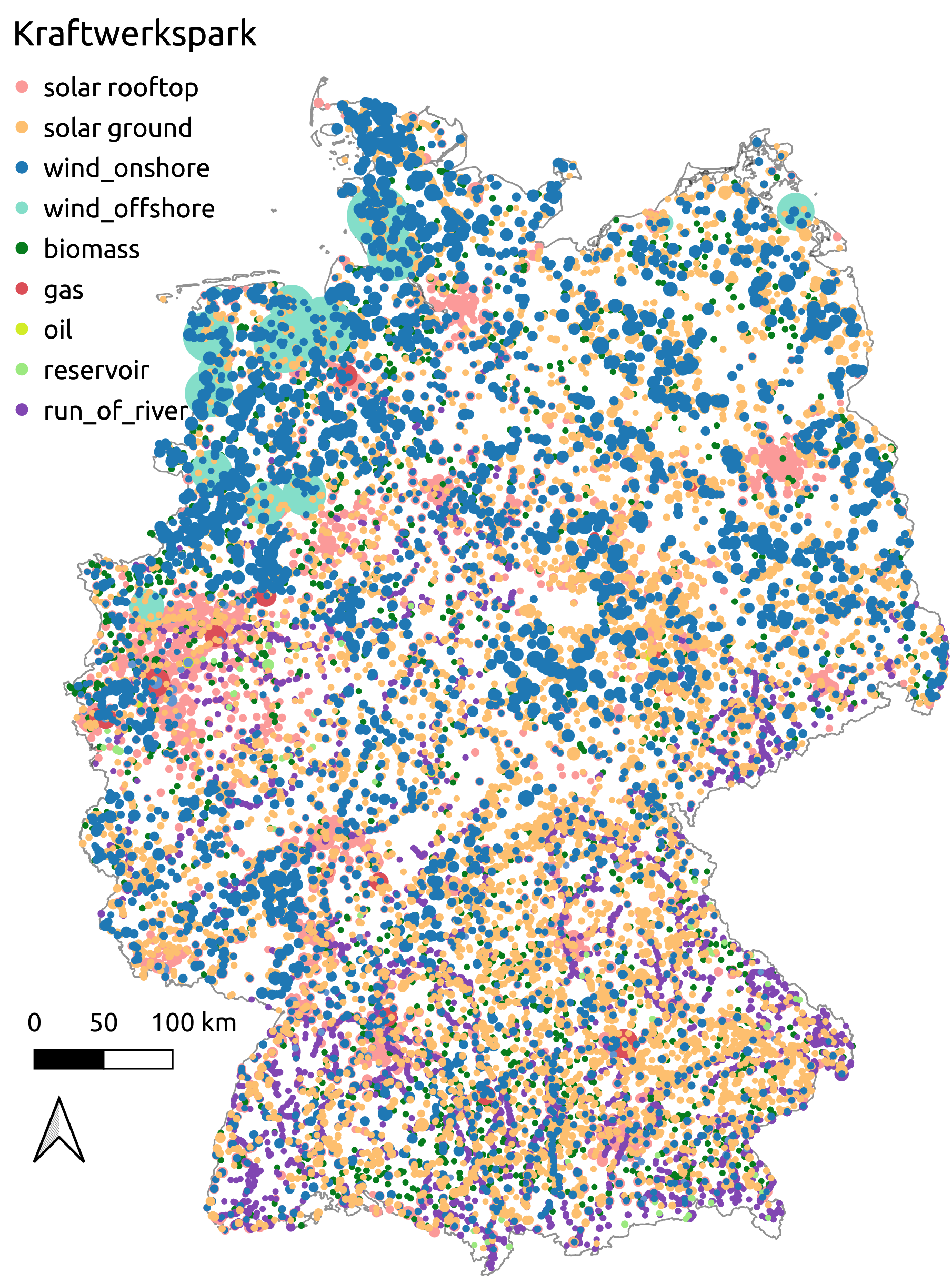
Generator park in the eGon2035 scenario

Onshore wind

The allocation of onshore wind power plants is implemented in the function insert which is part of the dataset PowerPlants. The following steps are conducted:

1. The sites and capacities of exisitng onshore wind parks are imported using MaStR data (see Marktstammdatenregister).

2. Potential areas for onshore wind parks are assumed to be areas With high mean wind speed, at the same time that some locations like protected natural areas or zones close to urban centers are discarted. Those areas are imported through the data bundle, see Data bundle).

3. The locations of existing parks and the potential areas are intersected with each other while considering a buffer around the locations of existing parks to find out where there are already parks at or close to potential areas. This results in a selection of potential areas.

4. The capacities of the existing parks matching potential areas are summed up and compared to the target values for the specific scenario per federal state (see Modeling concept and scenarios). The required expansion capacity is derived.

5. If expansion of wind onshore capacity is required, capacities are calculated depending on the area size of the formerly selected potential areas. 21.05 MW/km² and 16.81 MW/km² are used for federal states in the north and in the south of the country respectively. The resulting parks are therefore located on the selected potential areas.

6. The resulting capacities are compared to the target values for the specific scenario per federal state. If the target value is exceeded, a linear downscaling is conducted. If the target value is not reached yet, the remaining capacity is distributed linearly among the rest of the potential areas within the state.

Offshore wind

The allocation of offshore wind power plants is implemented in the function insert which is part of the dataset PowerPlants. The following steps are conducted:

1. A compilation of offshore wind parks for different scenarios created by NEP are extracted from the data bundle. See Data bundle. This data includes installed capacities, connection points (or a potential one for future power plants) and location. See figure Areas for offshore wind park in North and Baltic sea. Source: NEP.

2. Each connection point is matched to one of the substations previously created. Despite the fact that the generators are located in the sea, all the power generated by them will be injected into the grid through these substations, that in some cases can be several kilometers in land.

3. For the eGon100RE scenario, the installed capacities are scaled up in order to achieve the targed in Modeling concept and scenarios.

4. Each offshore wind power plant receives an hourly maximal generation capacity based on weather data for its own geographical location. Weather data provided by ERA5.

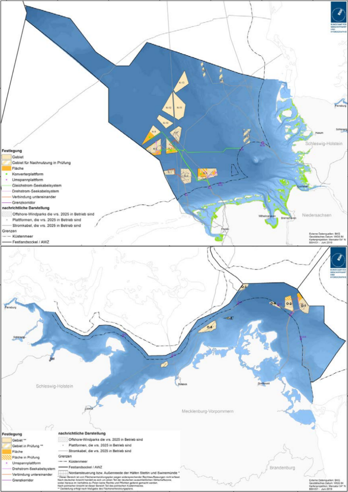
Areas for offshore wind park in North and Baltic sea. Source: NEP

PV ground mounted

The distribution of PV ground mounted is implemented in function insert which is part of the dataset PowerPlants. The following steps are conducted:

1. The sites and capacities of exisitng PV parks are imported using MaStR data (see Marktstammdatenregister).

2. Potential areas for PV ground mounted are assumed to be areas next to highways and railways as well as on agricultural land with a low degree of utilisation, as it can be seen in figure Example: sites of existing PV ground mounted parks and potential areas. Those areas (provided through the data bundle, see Data bundle) are imported while merging or disgarding small areas.

3. The locations of existing parks and the potential areas are intersected with each other while considering a buffer around the locations of existing parks to find out where there already are parks at or close to potential areas. This results in a selection of potential areas.

4. The capacities of the existing parks are considered and compared to the target values for the specific scenario per federal state (see Modeling concept and scenarios). The required expansion capacity is derived.

5. If expansion of PV ground mounted capacity is required, capacities are calculated depending on the area size of the formerly selected potential areas. The resulting parks are therefore located on the selected potential areas.

6. The resulting capacities are compared to the target values for the specific scenario per federal state. If the target value is exceeded, a linear downscaling is conducted. If the target value is not reached yet, the remaining capacity is distributed linearly among the rest of the potential areas within the state.

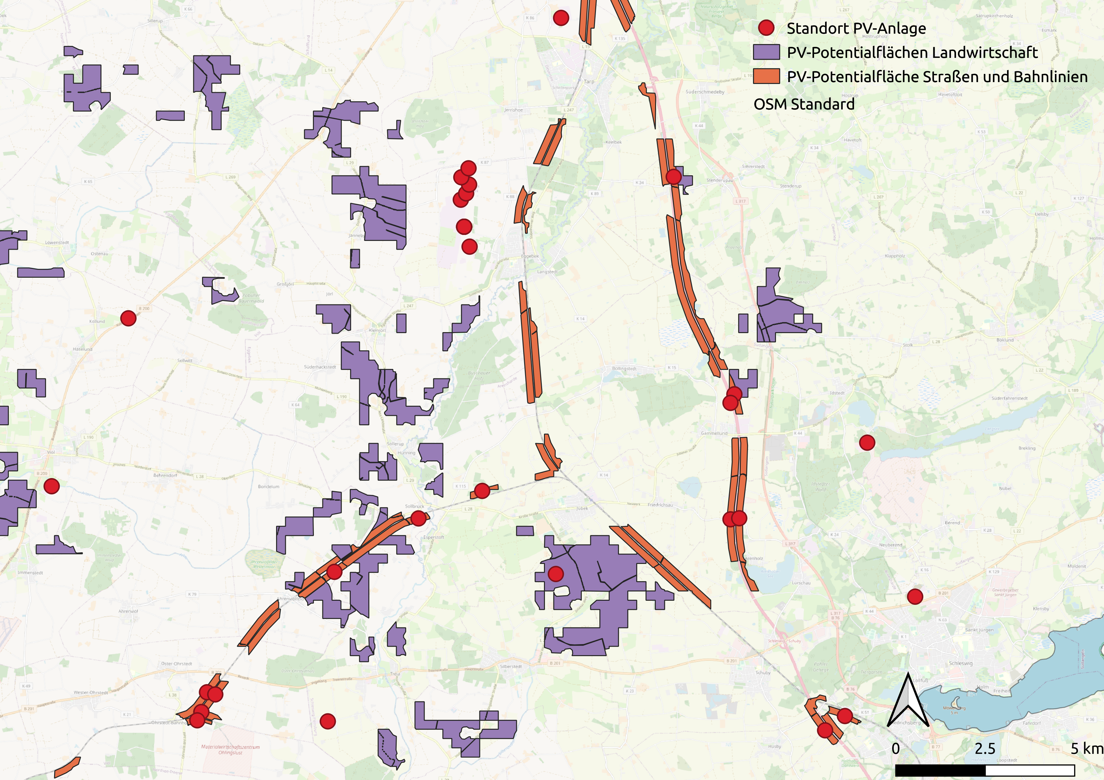
Example: sites of existing PV ground mounted parks and potential areas

PV rooftop

In a first step, the target capacity in the eGon2035 and eGon100RE scenarios is distributed to all MV grid districts linear to the residential and CTS electricity demands in the grid district (done in function pv_rooftop_per_mv_grid).

Afterwards, the PV rooftop capacity per MV grid district is disaggregated to individual buildings inside the grid district (done in function pv_rooftop_to_buildings). The basis for this is data from the MaStR, which is first cleaned and missing information inferred, and then allocated to specific buildings. New PV plants are in a last step added based on the capacity distribution from MaStR. These steps are in more detail described in the following.

MaStR data cleaning and inference:

• Drop duplicates and entries with missing critical data.

• Determine most plausible capacity from multiple values given in MaStR data.

• Drop generators that don’t have a plausible capacity (23.5 MW > P > 0.1 kW).

• Randomly and weighted add a start-up date if it is missing.

• Extract zip and municipality from ‘site’ given in MaStR data.

• Geocode unique zip and municipality combinations with Nominatim (1 sec delay). Drop generators for which geocoding failed or which are located outside the municipalities of Germany.

• Add some visual sanity checks for cleaned data.

Allocation of MaStR plants to buildings:

• Allocate each generator to an existing building from OSM or a synthetic building (see Building data).

• Determine the quantile each generator and building is in depending on the capacity of the generator and the area of the polygon of the building.

• Randomly distribute generators within each municipality preferably within the same building area quantile as the generators are capacity wise.

• If not enough buildings exist within a municipality and quantile additional buildings from other quantiles are chosen randomly.

Disaggregation of PV rooftop scenario capacities:

• The scenario data per federal state is linearly distributed to the MV grid districts according to the PV rooftop potential per MV grid district.

• The rooftop potential is estimated from the building area given from the OSM buildings.

• Grid districts, which are located in several federal states, are allocated PV capacity according to their respective roof potential in the individual federal states.

• The disaggregation of PV plants within a grid district respects existing plants from MaStR, which did not reach their end of life.

• New PV plants are randomly and weighted generated using the capacity distribution of PV rooftop plants from MaStR.

• Plant metadata (e.g. plant orientation) is also added randomly and weighted using MaStR data as basis.

Hydro

In the case of hydropower plants, a distinction is made between the carrier run-of-river and reservoir. The methods to distribute and allocate are the same for both carriers. In a first step all suitable power plants (correct carrier, valid geolocation, information about federal state) are selected and their installed capacity is scaled to meet the target values for the respective federal state and scenario. Information about the voltage level the power plants are connected to is obtained. In case no information is availabe the voltage level is identified using threshold values for the installed capacity (see assign_voltage_level). In a next step the correct grid connection point is identified based on the voltage level and geolocation of the power plants (see assign_bus_id) The resulting list of power plants it added to table EgonPowerPlants.

Biomass

The allocation of biomass-based power plants follows the same method as the one for hydro power plants and is performed in function insert_biomass_plants

Conventional

CHP

non-chp

In function allocate_conventional_non_chp_power_plants capacities for conventional power plants, which are no chp plants, with carrier oil and gas are allocated.

Gas turbines

The gas turbines, or open cycle gas turbines (OCGTs) allow the production of electricity from methane and are modelled with unidirectional PyPSA links, which connect methane buses to power buses.

The capacities of the gas turbines are invariable and considered as constant. The technical parameters (investment and marginal costs, efficiency, lifetime) comes from the PyPSA technology data [technoData].

In Germany, the gas turbines listed in the Netzentwicklungsplan [NEP2021] are matched to the Marktstammdatenregister in order to get their geographical coordinates in allocate_conventional_non_chp_power_plants. The matched units are then associated to the corresponding power and methane buses.

The implementation of gas turbines in the data model is detailed in the OpenCycleGasTurbineEtrago page of our documentation.

Warning

OCGT in Germany are still missing in eGon100RE: https://github.com/openego/eGon-data/issues/983

In the scenario eGon2035, the gas turbines capacities abroad comes from the TYNDP 2035 [TYNDP], the implementation is detailed in eGon2035.tyndp_gas_generation.

In the scenario eGon100RE the gas turbines capacities in the neighboring countries are taken directly from the PyPSA-eur-sec run.

Fuel cells

The fuel cells allow the production of electricity from hydrogen and are modelled with unidirectional PyPSA links, which connect hydrogen buses to power buses.

The data model contains the potentials of this technology, whose capacities are optimized. The technical parameters (investment and marginal costs, efficiency, lifetime) comes from the PyPSA technology data [technoData].

In the eGon2035 scenario, fuel cells are modelled at every hydrogen bus in Germany, as well as in the eGon100RE scenario. In eGon100RE, this technology is also modelled in the neighboring countries. In Germany, the potentials are generally not limited, except when the connected buses are located more than 500m far from each other. In this particular case, the potential has an upper limit of 1 MW.

The implementation of fuel cells in the data model is detailed in the power_to_h2 page of our documentation.

Heat

Heat demand of residential as well as commercial, trade and service (CTS) buildings can be supplied by different technologies and carriers. Within the data model creation, capacities of supply technologies are assigned to specific locations and their demands. The hourly dispatch of heat supply is not part of the data model, but a result of the grid optimization tools.

In general, heat supply can be divided into three categories which include specific technologies: residential and CTS buildings in a district heating area, buildings supplied by individual heat pumps, and buildings supplied by conventional gas boilers. The shares of these categories are taken from external sources for each scenario.

Heat demands of different supply categories

	District heating	Individual heat pumps	Individual gas boilers
eGon2035	69 TWh	27.24 TWh	390.78 TWh
eGon100RE	61.5 TWh	311.5 TWh	0 TWh

The following subsections describe the heat supply methodology for each category.

District heating

First, district heating areas are defined for each scenario based on existing district heating areas and an overall district heating share per scenario. To reduce the model complexity, district heating areas are defined per Census cell, either all buildings within a cell are supplied by district heat or none. The first step of the extraction of district heating areas is the identification of Census cells with buildings that are currently supplied by district heating using the building dataset of Census. All Census cells where more than 30% of the buildings are currently supplied by district heat are defined as cells inside a district heating area. The identified cells are then summarized by combining cells that have a maximum distance of 500m.

Second, additional Census cells are assigned to district heating areas considering the heat demand density. Assuming that new district heating grids are more likely in cells with high demand, the remaining Census cells outside of a district heating grid are sorted by their demands. Until the pre-defined national district heating demand is met, cells from that list are assigned to district heating areas. This can also result in new district heating grids which cover only a few Census cells.

To avoid unrealistic large district heating grids in areas with many cities close to each other (e.g. the Ruhr Area), district heating areas with an annual demand > 4 TWh are split by NUTS3 boundaries.

The implementation of the district heating area demarcation is done in DistrictHeatingAreas, the resulting data is stored in the tables demand.egon_map_zensus_district_heating_areas and demand.egon_district_heating_areas. The resulting district heating grids for the scenario eGon2035 are visualized in figure Defined district heating grids in scenario eGon2035, which also includes a zoom on the district heating grid in Berlin.

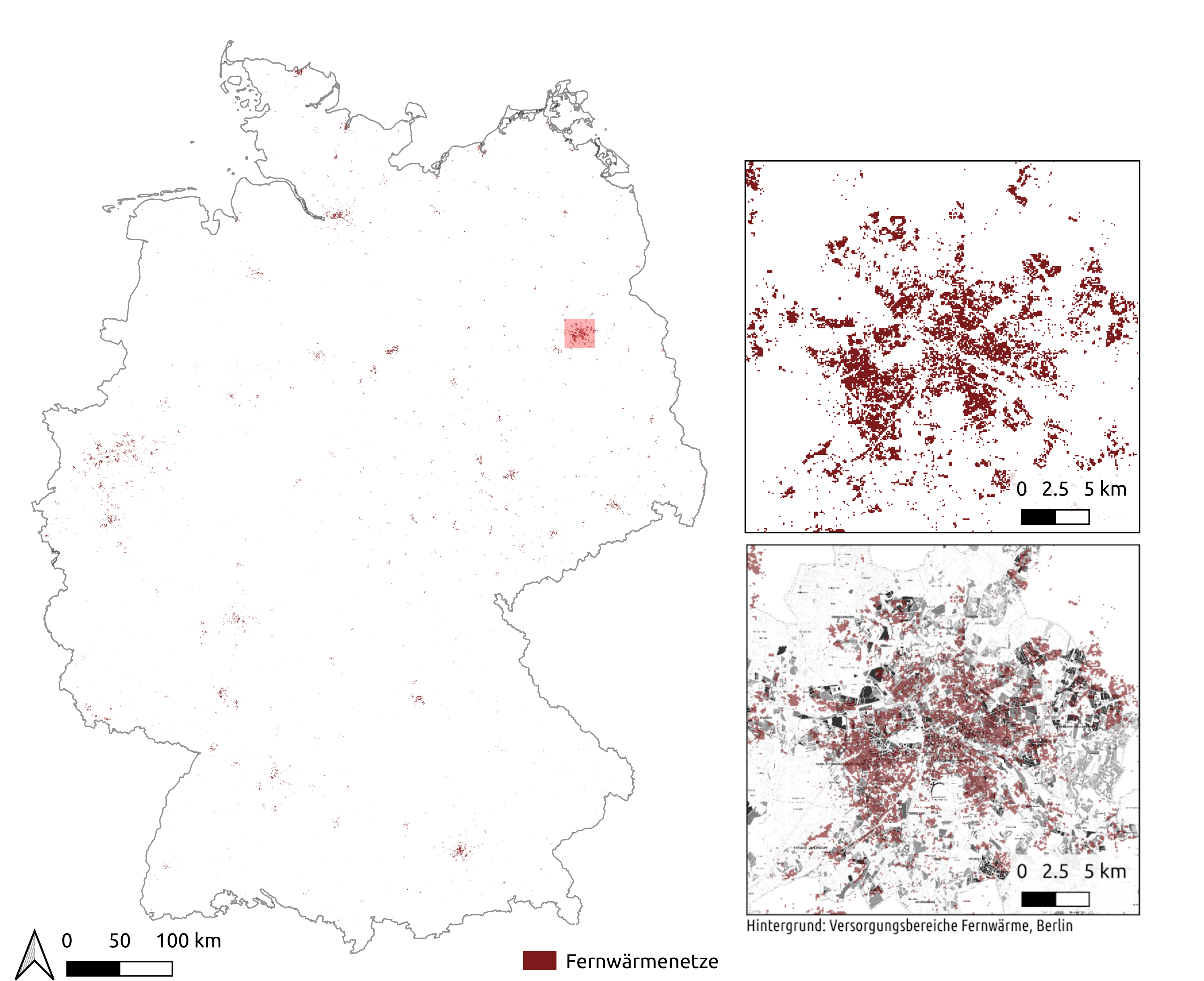
Defined district heating grids in scenario eGon2035

The national capacities for each supply technology are taken from the Grid Development Plan (GDP) for the scenario eGon2035, in the eGon100RE scenario they are the result of the pypsa-eur-sec run. The distribution of the capacities to district heating grids is done similarly based on [FfE2017], which is also used in the GDP. The basic idea of this method is to use a cascade of heat supply technologies until the heat demand can be covered.

1. Combined heat and power (CHP) plants are assigned to nearby district heating grids first. Their location and thermal capacities are from Marktstammdatenregister [MaStR]. To identify district heating grids that need additional suppliers, the remaining annual heat demand is calculated using the thermal capacities of the CHP plants and assumed full load hours.

2. Large district heating grids with an annual demand that is higher than 96GWh can be supplied by geothermal plants, in case of an intersection of geothermal potential areas and the district heating grid. Smaller district heating grids can be supplied by solar thermal power plants. The national capacities are distributed proportionally to the remaining heat demands. After assigning these plants, the remaining heat demands are reduced by the thermal output and assumed full load hours.

3. Next, the national capacities for central heat pumps and resistive heaters are distributed to all district heating areas proportionally to their remaining demands. Heat pumps are modeled with a time-dependent coefficient of performance (COP) depending on the temperature data. The COP is determined in function heat_pump_cop as part of the RenewableFeedin dataset and written to database table supply.egon_era5_renewable_feedin.

4. In the last step, gas boilers are assigned to every district heating grid regardless of the remaining demand. In the optimization, this can be used as a fall-back option to not run into infeasibilities.

The distribution of CHP plants for different carriers is shown in figure Spatial distribution of CHP plants in scenario eGon2035.

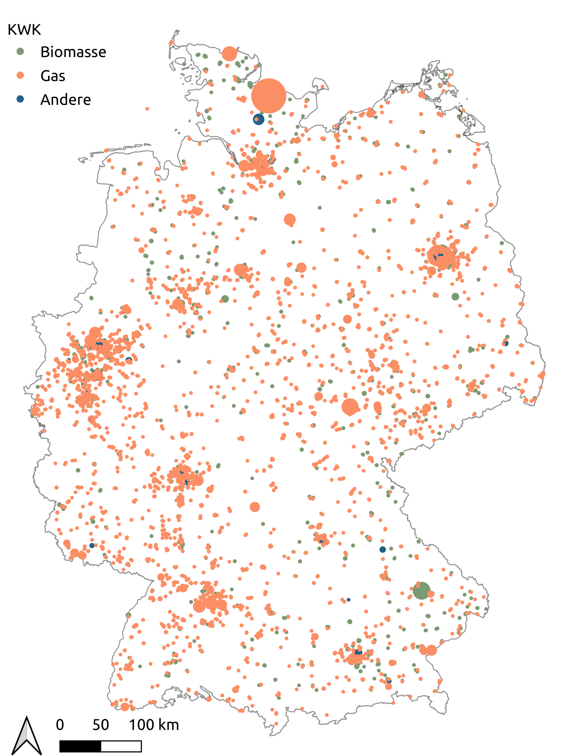
Spatial distribution of CHP plants in scenario eGon2035

Individual heat pumps

Heat pumps supplying individual buildings are first distributed to each medium-voltage grid district. These capacities are later on further disaggregated to single buildings. Similar to central heat pumps, individual heat pumps are modeled with a time-dependent coefficient of performance depending on the temperature data.

The distribution of the national capacities to each medium-voltage grid district is proportional to the heat demand outside of district heating grids.

The heat pump capacity per MV grid district is further disaggregated to individual buildings based on the building’s peak heat demand. For the eGon2035 scenario this is conducted in the dataset HeatPumps2035 and for the eGon100RE scenario in the dataset HeatPumps2050. The heat pump capacity per building is for both scenarios written to database table demand.egon_hp_capacity_buildings. The peak heat demand per building is written to database table demand.egon_building_heat_peak_loads.

To disaggregate the total heat pump capacity per MV grid, first, the minimum required heat pump capacity per building is determined. To this end, an approach from the network development plan (pp.46-47) is used where the heat pump capacity of a building is calculated by multiplying the peak heat demand of the building by a minimum assumed COP of 1.7 and a flexibility factor of 24/18 that is taking into account that power supply of heat pumps can be interrupted for up to six hours by the local distribution grid operator.

After the determination of the minimum required heat pump capacity per building, the total heat pump capacity per MV grid district is distributed to buildings inside the grid district based on the minimum required heat pump capacity. In the eGon2035 scenario, heat pumps and gas boilers can be used for individual heating. Therefore, it needs to be chosen which buildings are assigned a heat pump and which are assigned a gas boiler. To this end, buildings are randomly chosen until the MV grid’s total heat pump capacity is reached (see determine_buildings_with_hp_in_mv_grid). Buildings with PV rooftop plants are set to be more likely to be assigned a heat pump. In case the minimum heat pump capacity of all chosen buildings is smaller than the total heat pump capacity of the MV grid but adding another building would exceed the total heat pump capacity of the MV grid, the remaining capacity is distributed to all buildings with heat pumps proportionally to their respective minimum required heat pump capacity.

In the eGon100RE scenario, heat pumps are assumed to be the only technology for individual heating, wherefore all buildings outside of district heating areas are assigned a heat pump. The total heat pump capacity in the MV grid district is distributed to all buildings with individual heating proportionally to the minimum required heat pump capacity. To assure that the heat pump capacity per MV grid district, that is in case of the eGon100RE scenario optimised using PyPSA-EUR, is sufficient to meet the minimum required heat pump capacity of each building, the minimum required heat pump capacity per MV grid district is given as an input to the PyPSA-EUR optimisation. Therefore, the minimum heat pump capacity per building in the eGon100RE scenario is calculated and aggregated per grid district in the dataset HeatPumpsPypsaEurSec and written to csv file input-pypsa-eur-sec/minimum_hp_capacity_mv_grid_100RE.csv.

Drawbacks and limitations as well as challenges of the determination of the minimum required heat pump capacity and the disaggregation to individual buildings are discussed in the respective dataset docstrings of HeatPumps2035, HeatPumps2050 and HeatPumpsPypsaEurSec.

Individual gas boilers

All residential and CTS buildings that are neither supplied by a district heating grid nor an individual heat pump are supplied by gas boilers. The demand time series of these buildings are multiplied by the efficiency of gas boilers and aggregated per methane grid node.

All heat supply categories are implemented in the dataset HeatSupply. The data is stored in the tables demand.egon_district_heating and demand.egon_individual_heating.

Gas

Methane is directly produced, what is modelled through PyPSA generators. These generators have invariable capacities.

In the scenario eGon2035 the production of biogas as well as the production of natural gas are represented. In the scenario eGon100RE, only biogas is produced. These production potentials are considered as constant.

In Germany, the extraction potentials of natural gas are taken from the SciGRID_gas data [SciGRID_gas]. They are only used in the eGon2035 scenario. The biogas production potentials are from the Biogaspartner Einspeiseatlas [Einspeiseatlas] and are in both scenarios. The spatial repartition of the methane production potentials in Germany is represented in the figure below: left, the biogas production potentials (in green) and right the natural gas production potential (in grey).

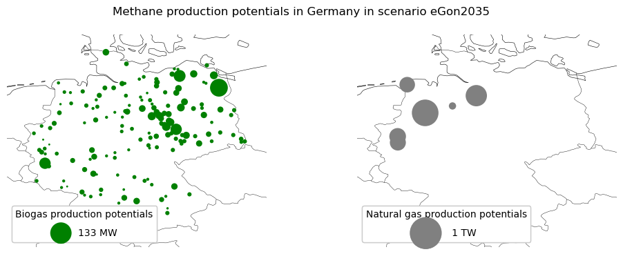
In the scenario eGon2035, the German production over the year of natural gas and of biogas is limited by values from the Netzentwicklungsplan Gas 2020–2030 [NEP_gas] (36 TWh natural gas and 10 TWh biogas). In the scenario eGon100RE, the German biogas production is limited by a value calculated in the PyPSA-eur-sec run (14.45 TWh).

The implementation of these data is detailed in the ch4_prod page of our documentation.

In the neighboring countries, the methane production potentials includes biogas and natural gas potential (with data from the TYNDP), as well as LNG terminals import potential (with data from SciGRID_gas). The implementation of these data is detailed in the gas_neighbours.eGon2035 page of our documentation.

In the scenario eGon100RE, the biogas production potentials of the neighboring countries are taken directly from the PyPSA-eur-sec run.

The following table summarize the multiple sources used to model the methane production potentials in the both scenarios.

References overview of the methane production potentials

		eGon2035		eGon100RE
		Natural gas	Biogas	Biogas
Germany	Regionalization	SciGRID_gas	Biogaspartner Einspeiseatlas	Biogaspartner Einspeiseatlas
	Max production over the year	NEP Gas	NEP Gas	PyPSA-eur-sec run
Neighbouring countries		TYNDP Also includes LNG terminal import potentials from SciGRID_gas		PyPSA-eur-sec run

The methanation is the production of methane from hydrogen and the Steam Methane Reforming (SMR) allows the reverse process: producing hydrogen with methane.

Methanation and SMR are modelled with unidirectional PyPSA links, which connect methane buses to hydrogen buses. The data model contains the potentials of these technologies, whose capacities are optimized. The technical parameters (investment and marginal costs, efficiency, lifetime) comes from the PyPSA technology data [technoData].

In both scenarios, methanation and SMR are modelled at every methane bus in Germany. Each one corresponding to a H2_grid bus, only these hydrogen buses do have these technologies attached (in other words, H2_saltcavern buses are not involved in methanation and SMR links). In both scenarios, the potentials are not limited. In the eGon100RE scenario, these technologies are also modelled in the neighboring countries.

The implementation of methanation and SMR in the data model is detailed in the h2_to_ch4 page of our documentation.

The hydrogen feedin is modelled only in the scenario eGon2035 and corresponds to the direct introduction of hydrogen into the methane grid. The hydrogen feedin is modelled with unidirectional PyPSA links, which connect hydrogen buses to methane buses. This transformation is possible at every methane bus with a invariable capacity calculated as 15% of the sum of the methane pipeline capacities at this specific bus.

Warning

We found out that this very simplified model does not work good enough because the constant capacity of the feedin links does not account for the flow in the pipelines, which varies in the times.

The implementation of hydrogen feedin in the data model is detailed in the h2_to_ch4 page of our documentation.

The electrolysis, the production of hydrogen from electricity is modelled with unidirectional PyPSA links, which connect power buses to hydrogen buses.

The data model contains the potentials of this technology, whose capacities are optimized. The technical parameters (investment and marginal costs, efficiency, lifetime) comes from the PyPSA technology data [technoData].

In the eGon2035 scenario, electrolysis is modelled at every hydrogen bus in Germany, as well as in the eGon100RE scenario. In eGon100RE, this technology is also modelled in the neighboring countries. In Germany, the potentials are generally not limited, except when the connected buses are located more than 500m far from each other. In this particular case, the potential has an upper limit of 1 MW.

The implementation of electrolysis in the data model is detailed in the power_to_h2 page of our documentation.

Flexibility options

Different flexibility options are part of the model and can be utilized in the optimization of the energy system. Therefore detailed information about flexibility potentials and their distribution are needed. The considered technologies described in the following chapters range from different storage units, through dynamic line rating to Demand-Side-Management measures.

Demand-Side Management

Demand-side management (DSM) potentials are calculated in function dsm_cts_ind_processing. Potentials relevant for the high and extra-high voltage grid are identified in the function dsm_cts_ind, potentials within the medium- and low-voltage grids are determined within the function dsm_cts_ind_individual in a higher spatial resolution. All this is part of the dataset DsmPotential. The implementation is documented in detail within the following student work (in German): [EsterlDentzien].

Loads eligible to be shifted are assumed within industrial loads and loads from Commercial, Trade and Service (CTS). Therefore, load time series from these sectors are used as input data (see section ref:elec_demand-ref). Shiftable shares of loads mainly derive from heating and cooling processes and selected energy-intensive industrial processes (cement production, wood pulp, paper production, recycling paper). Technical and sociotechnical constraints are considered using the parametrization elaborated in [Heitkoetter]. An overview over the resulting potentials for scenario eGon2035 can be seen in figure Aggregated DSM potential in Germany for scenario eGon2035. The table below summarizes the aggregated potential for Germany per scenario. As the annual conventional electrical loads are assumed to be lower in the scenario eGon100RE, also the DSM potential decreases compared to the scenario eGon2035.

Aggregated DSM potential in Germany for scenario eGon2035

Aggregated DSM Potential for Germany

	CTS	Industry
eGon2035	1.2 GW	150 MW
eGon100RE	900 MW	150 MW

DSM is modelled following the approach of [Kleinhans]. DSM components are created wherever respective loads are seen. Minimum and maximum shiftable power per time step depict time-dependent charging and discharging power of a storage-equivalent buffers. Time-dependent capacities of those buffers account for the time frame of management bounding the period within which the shifting can be conducted. Figure Time-dependent DSM potential at one exemplary bus shows the resulting potential at one exemplary bus.

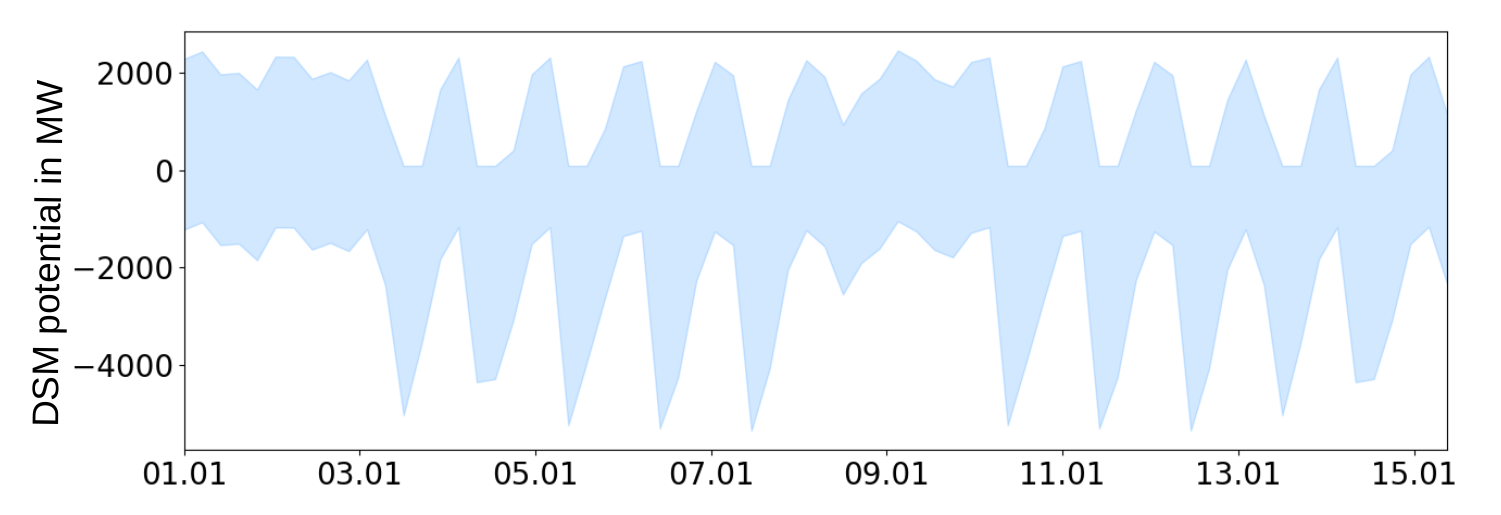
Time-dependent DSM potential at one exemplary bus

Dynamic line rating

To calculate the transmission capacity of each transmission line in the model, the procedure suggested in the Principles for the Expansion Planning of the German Transmission Network [NEP2021a] where used:

1. Import the temperature and wind temporal raster layers from ERA-5. Hourly resolution data from the year 2011 was used. Raster resolution latitude-longitude grids at 0.25° x 0.25°.

2. Import shape file for the 9 regions proposed by the Principles for the Expansion Planning. See Figure 1.

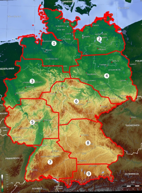
Figure 1: Representative regions in Germany for DLR analysis [NEP2021a]

3. Find the lowest wind speed in each region. To perform this, for each independent region, the wind speed of every cell in the raster layer should be extracted and compared. This procedure is repeated for each hour in the year 2011. The results are the 8760 lowest wind speed per region.

4. Find the highest temperature in each region. To perform this, for each independent region, the temperature of every cell in the raster layer should be extracted and compared. This procedure is repeated for each hour in the year 2011. The results are the 8760 maximum temperature per region.

5. Calculate the maximum capacity for each region using the parameters shown in Figure 2.

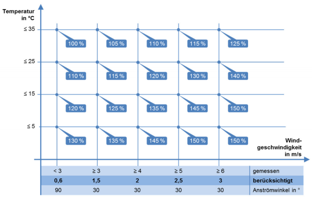
Figure 2: transmission capacity based on max temperature and min wind speed [NEP2021a]

6. Assign the maximum capacity of the corresponding region to each transmission line inside each one of them. Crossborder lines and underground lines receive no values. It means that their capacities are static and equal to their nominal values. Lines that cross borders between regions receive the lowest capacity per hour of the regions containing the line.

Flexible charging of EVs

The flexibility potential of EVs is determined on the basis of the trip data created with SimBEV (see Motorized individual travel). It is assumed, that only charging at private charging points, comprising charging points at home and at the workplace, can be flexibilized. Public fast (e.g. gas stations) and slow charging (e.g. schools and shopping facilities) stations are assumed not to provide demand-side flexibility. Further, vehicle-to-grid is not considered and it is assumed that charging can only be shifted within a charging event. Shifting charging demand to a later charging event, for example from charging at work during working hours to charging at home in the evening, is therefore not possible. In the generation of the trip data itself it is already considered, that EVs are not charged everytime a charging point is available, but only if a certain lower state of charge (SoC) is reached or the energy level is not sufficient for the next ride.

In eTraGo, the flexibility of the EVs is modeled using a storage model based on [Brown2018] and [Wulff2020]. The used model is visualised in the upper right in figure Workflow to set up charging demand data for MIT in the eGon2035 scenario. Its parametrization is for both the eGon2035 and eGon100RE scenario conducted in the MotorizedIndividualTravel dataset in the function generate_load_time_series. The model consists of loads for static driving demands and stores for the fleet’s batteries. The stores are constrained by hourly lower and upper SoC limits. The lower SoC limit represents the inflexible charging demand while the SoC band between the lower and upper SoC limit represents the flexible charging demand. Further, the charging infrastructure is represented by unidirectional links from electricity buses to EV buses. Its maximum charging power per hour is set to the available charging power of grid-connected EVs.

In eDisGo, the flexibility potential for controlled charging is modeled using so-called flexibility bands. These bands comprise an upper and lower power band for the charging power and an upper and lower energy band for the energy to be recharged for each charging point in an hourly resolution. These flexibility bands are not set up in eGon-data but in eDisGo, using the trip data from eGon-data. For further information on the flexibility bands see eDisGo documentation.

Battery stores

Battery storage units comprise home batteries and larger, grid-supportive batteries. National capacities for home batteries arise from external sources, e.g. the Grid Development Plan for the scenario eGon2035, whereas the capacities of large-scale batteries are a result of the grid optimization tool eTraGo.

Home battery capacities are first distributed to medium-voltage grid districts (MVGD) and based on that further disaggregated to single buildings. The distribution on MVGD level is done proportional to the installed capacities of solar rooftop power plants, assuming that they are used as solar home storage.

Potential large-scale batteries are included in the data model at every substation. The data model includes technical and economic parameters, such as efficiencies and investment costs. The energy-to-power ratio is set to a fixed value of 6 hours. Other central parameters are given in the following table

Parameters of batteries for scenario eGon2035

	Value	Sources
Efficiency store	98 %	[DAE_store]
Efficiency dispatch	98 %	[DAE_store]
Standing loss	0 %	[DAE_store]
Investment costs	838 €/kW	[DAE_store]
Home storage units	16.8 GW	[NEP2021]

On transmission grid level, distinguishing between home batteries and large-scale batteries was not possible. Therefore, the capacities of home batteries were set as a lower boundary of the large-scale battery capacities. This is implemented in the dataset StorageEtrago, the data for batteries in the transmission grid is stored in the database table grid.egon_etrago_storage.

Gas stores

In both scenarios is there the option to store hydrogen. In the scenario eGon2035, these potentials are modelled only in Germany, because the hydrogen sector is not modelled in the neighboring countries. Hydrogen is stored either in steel tanks (overground storage) or in saltcavern (underground storage), which are modelled by PyPSA stores. The technical parameters (investment and marginal costs, efficiency, lifetime) comes from the PyPSA technology data [technoData]. The steel tank storage potentials are not limited. On the contrary, the saltcavern storage potentials do have an upper boundary.

The saltcavern potentials are located at the intersection between the power substations and the adapted saltcavern surface areas, defined in the InSpEE-DS report from the Bundesanstalt für Geowissenschaften und Rohstoffe [BGR]. These potentials, identical in the both scenarios, are represented in the figure below.

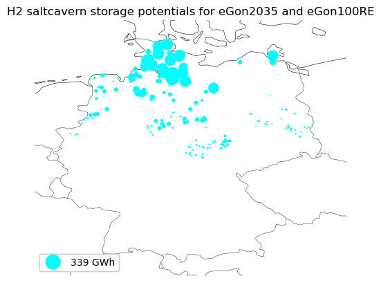
The implementation of these data is detailed in the hydrogen_etrago.storage page of our documentation.

In eGon100RE, the retrofitted hydrogen grid can also be used as storage, with unvariable capacity. This implementation is detailed in the grid_storage page of our documentation.

In the scenario eGon100RE the hydrogen storage potentials in the neighboring countries are taken directly from the PyPSA-eur-sec run.

The methane stores are modelled as PyPSA stores and they are invariable. In Germany, two types of methane stores are modelled:

• the underground caverns: capacities from SciGRID_gas [SciGRID_gas],

• the storage capacity of the German gas grid.

The storage capacity of the gas grid (130 GWh according to the Bundesnetzagentur [Bna]) is uniformly distributed between all the methane nodes in Germany in the scenario eGon2035. In the scenario eGon100RE, the retrofitted hydrogen grid take a share of this storage capacity over.

The implementation of the methane storage in the data model is detailed in the ch4_storages page of our documentation.

In the neighboring countries, the methane store capacities from SciGRID_gas [SciGRID_gas] are used in the eGon2035 scenario and data from PyPSA-eur-sec are used in the eGon100RE scenario.

Heat stores

The heat sector can provide flexibility through stores that allow shifting energy in time. The data model includes hot water tanks as heat stores in individual buildings and pit thermal energy storage for district heating grids (further described in District heating).

Within the data model, potential locations as well as technical and economic parameters of these stores are defined. The installed store and (dis-)charging capacities are part of the grid optimization methods that can be performed by eTraGo. The power-to-energy ratio is not predefined but a result of the optimization, which allows to build heat stores with various time horizons.

Individual heat stores can be built in every building with an individual heat pump. Central heat stores can be built next to district heating grids. There are no maximum limits for the energy output as well as (dis-)charging capacities implemented yet.

Central cost assumptions for central and decentral heat stores are listed in the table below. The parameters can differ for each scenario in order to include technology updates and learning curves. The table focuses on the scenario eGon2035.

Parameters of heat stores

	Technology	Costs for store capacity	Costs for (dis-)charging capacity	Round-trip efficiency	Sources
District heating	Pit thermal energy storage	0.51 EUR / kWh	0 EUR / kW	70 %	[DAE_store]
Buildings with heat pump	Water tank	1.84 EUR / kWh	0 EUR / kW	70 %	[DAE_store]

The heat stores are implemented as a part of the dataset HeatEtrago, the data is written into the tables grid.egon_etrago_bus, grid.egon_etrago_link and grid.egon_etrago_store.

Published data