Heat demands comprise space heating and dirinking hot water demands from residential and comertial trade and service (CTS) buildings. Process heat demands from the industry are, depending on the required temperature level, modelled as electrcity, hydrogen or methane demand.

The spatial distribution of annual heat demands is taken from the Pan-European Thermal Altlas version 5.0.1 [Peta]. This source provides data on annual european residential and CTS heat demands per hectar cell for the year 2015. In order to model future demands, the demand distribution extracted by Peta is then scaled to meet a national annual demand from external sources. The following national demands are taken for the selected scenarios:

Heat demands per sector and scenario

	Residential sector	CTS sector	Sources
eGon2035	379 TWh	122 TWh	[Energiereferenzprognose]
eGon100RE	284 TWh	89 TWh	[Energiereferenzprognose]

The resulting data is stored in the database table demand.egon_peta_heat. The implementation of these dataprocessing steps can be found in HeatDemandImport.

Figure Spatial distribution of residential heat demand in scenario eGon2035 shows the distribution of residential heat demands for scenario eGon2035, categorized for different levels of annual demands.

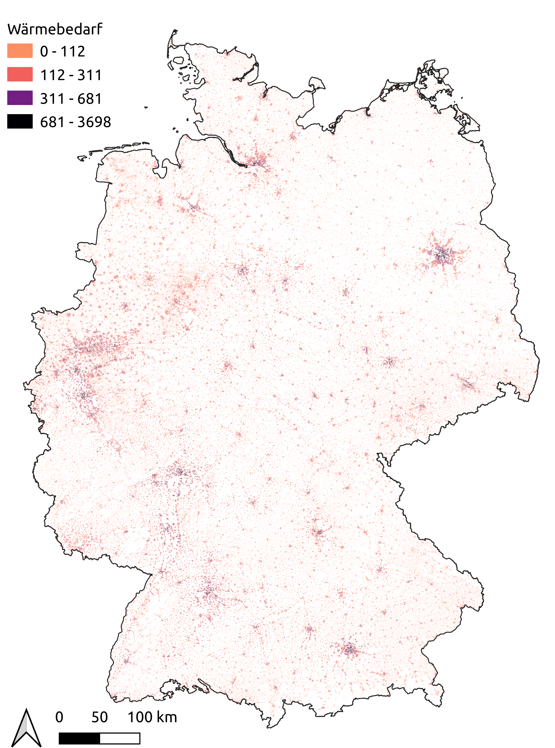
Spatial distribution of residential heat demand in scenario eGon2035

Afterwards, the annual heat demands are used to create hourly heat demand profiles. For residential heat demand profiles a pool of synthetical created bottom-up demand profiles is used. Depending on the mean temperature per day, these profiles are randomly assigned to each residential building. The methodology is described in detail in [Buettner2022].

Data on residential heat demand profiles is stored in the database within the tables demand.egon_heat_timeseries_selected_profiles, demand.egon_daily_heat_demand_per_climate_zone, boundaries.egon_map_zensus_climate_zones. To create the profiles for a selected buidling, these tables have to be combined, e.g. like this:

SELECT (b.demand/f.count * UNNEST(e.idp) * d.daily_demand_share)*1000 AS demand_profile
FROM (SELECT * FROM demand.egon_heat_timeseries_selected_profiles,
UNNEST(selected_idp_profiles) WITH ORDINALITY as selected_idp) a
JOIN demand.egon_peta_heat b
ON b.zensus_population_id = a.zensus_population_id
JOIN boundaries.egon_map_zensus_climate_zones c
ON c.zensus_population_id = a.zensus_population_id
JOIN demand.egon_daily_heat_demand_per_climate_zone d
ON (c.climate_zone = d.climate_zone AND d.day_of_year = ordinality)
JOIN demand.egon_heat_idp_pool e
ON selected_idp = e.index
JOIN (SELECT zensus_population_id, COUNT(building_id)
FROM demand.egon_heat_timeseries_selected_profiles
GROUP BY zensus_population_id
) f
ON f.zensus_population_id = a.zensus_population_id
WHERE a.building_id = SELECTED_BUILDING_ID
AND b.scenario = 'eGon2035'
AND b.sector = 'residential';

Exemplary resulting residential heat demand time series for a selected day in winter and summer considering different aggregation levels are visualized in figures Temporal distribution of residential heat demand for a selected day in winter and Temporal distribution of residential heat demand for a selected day in summer.

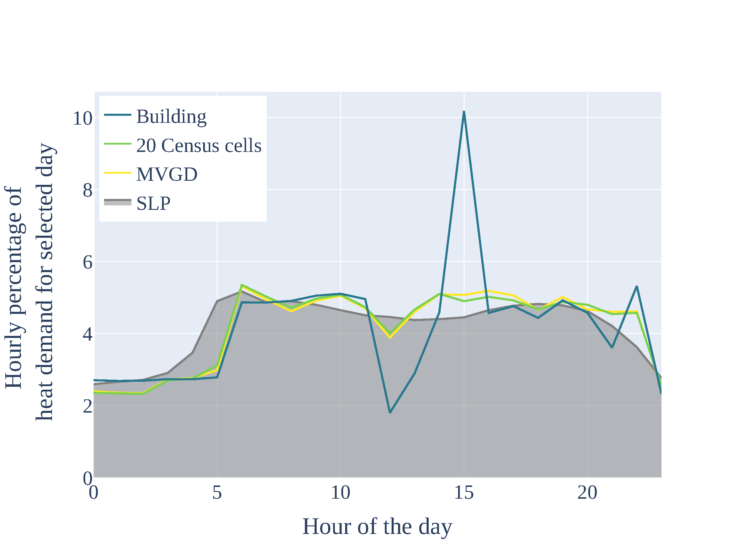
Temporal distribution of residential heat demand for a selected day in winter

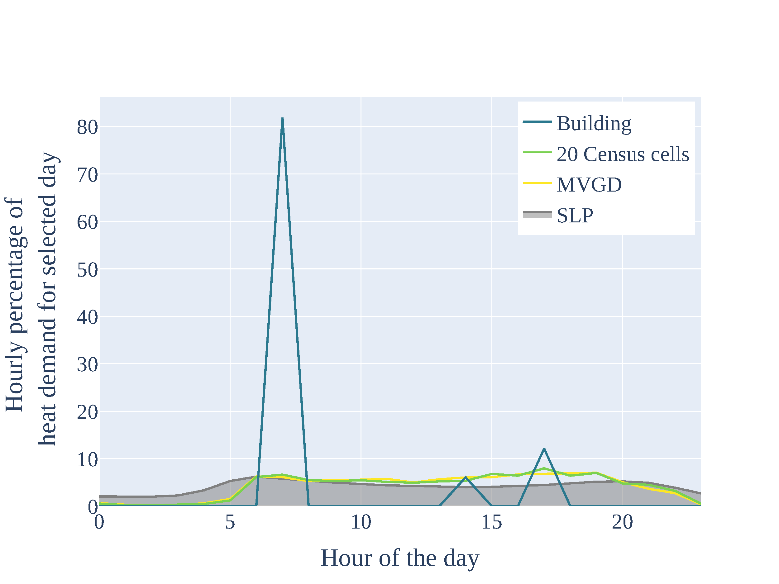
Temporal distribution of residential heat demand for a selected day in summer

The temporal disaggregation of CTS heat demand is done using Standard Load Profiles Gas from demandregio [demandregio] considering different profiles per CTS branch.

The heat demand time series for both sectors creation is done in the Dataset HeatTimeSeries.