The electrical power plants park, including data on geolocations, installed capacities, etc.
for the different scenarios is set up in the dataset
PowerPlants.
Main inputs into the dataset are target capacities per technology and federal state in each scenario (see Modeling concept and scenarios) as well as the MaStR (see Marktstammdatenregister), OpenStreetMap (see OpenStreetMap) and potential areas (provided through the data bundle, see Data bundle) to distribute the generator capacities within each federal state region. The approach taken to distribute the target capacities within each federal state differs for the different technologies and is described in the following. The final distribution in the eGon2035 scenario is shown in figure Generator park in the eGon2035 scenario.
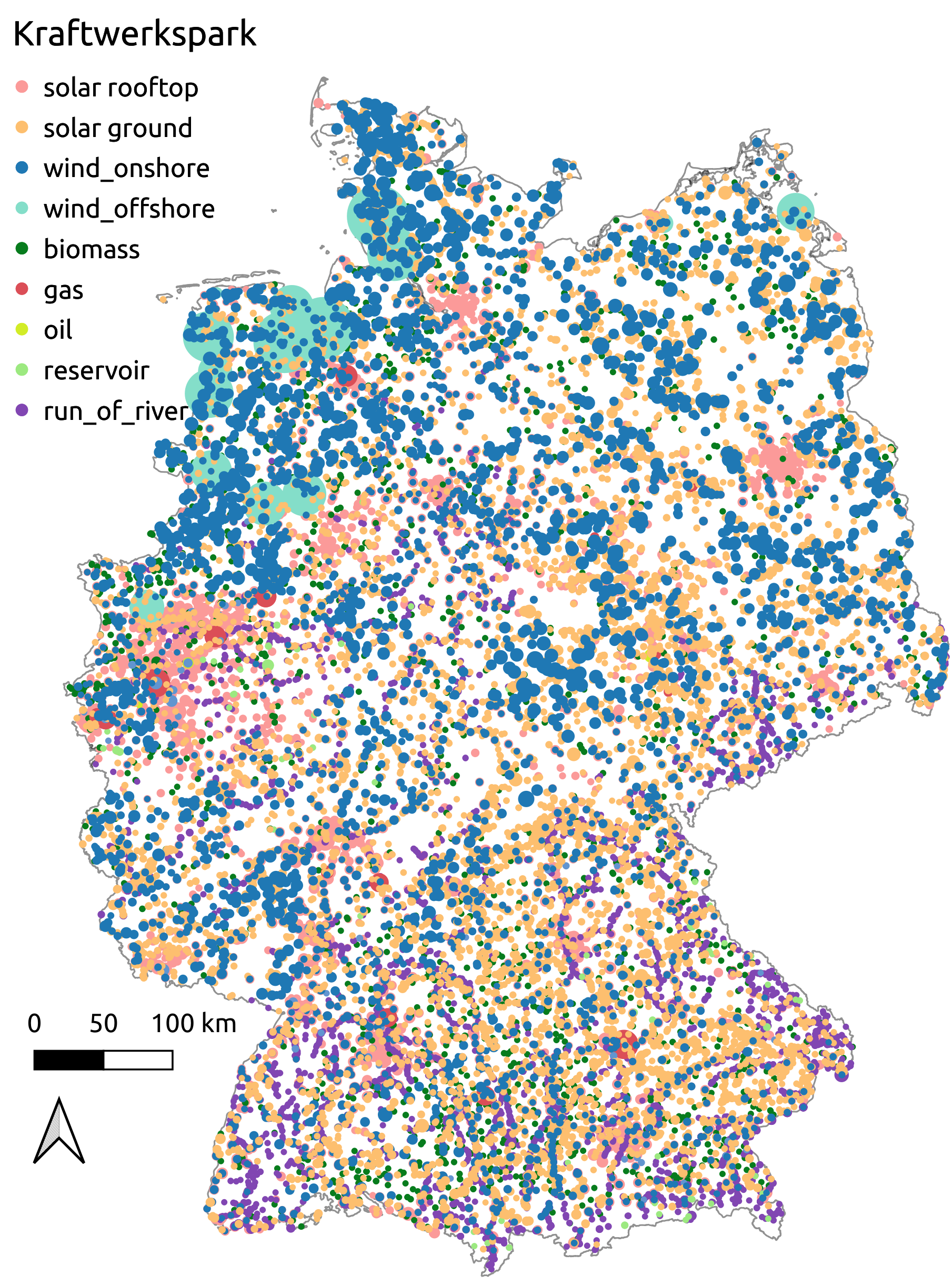
Generator park in the eGon2035 scenario
Onshore wind
The allocation of onshore wind power plants is implemented in the function insert
which is part of the dataset PowerPlants.
The following steps are conducted:
The sites and capacities of exisitng onshore wind parks are imported using MaStR data (see Marktstammdatenregister).
Potential areas for onshore wind parks are assumed to be areas With high mean wind speed, at the same time that some locations like protected natural areas or zones close to urban centers are discarted. Those areas are imported through the data bundle, see Data bundle).
The locations of existing parks and the potential areas are intersected with each other while considering a buffer around the locations of existing parks to find out where there are already parks at or close to potential areas. This results in a selection of potential areas.
The capacities of the existing parks matching potential areas are summed up and compared to the target values for the specific scenario per federal state (see Modeling concept and scenarios). The required expansion capacity is derived.
If expansion of wind onshore capacity is required, capacities are calculated depending on the area size of the formerly selected potential areas. 21.05 MW/km² and 16.81 MW/km² are used for federal states in the north and in the south of the country respectively. The resulting parks are therefore located on the selected potential areas.
The resulting capacities are compared to the target values for the specific scenario per federal state. If the target value is exceeded, a linear downscaling is conducted. If the target value is not reached yet, the remaining capacity is distributed linearly among the rest of the potential areas within the state.
Offshore wind
The allocation of offshore wind power plants is implemented in the function insert
which is part of the dataset PowerPlants.
The following steps are conducted:
A compilation of offshore wind parks for different scenarios created by NEP are extracted from the data bundle. See Data bundle. This data includes installed capacities, connection points (or a potential one for future power plants) and location. See figure Areas for offshore wind park in North and Baltic sea. Source: NEP.
Each connection point is matched to one of the substations previously created. Despite the fact that the generators are located in the sea, all the power generated by them will be injected into the grid through these substations, that in some cases can be several kilometers in land.
For the eGon100RE scenario, the installed capacities are scaled up in order to achieve the targed in Modeling concept and scenarios.
Each offshore wind power plant receives an hourly maximal generation capacity based on weather data for its own geographical location. Weather data provided by ERA5.
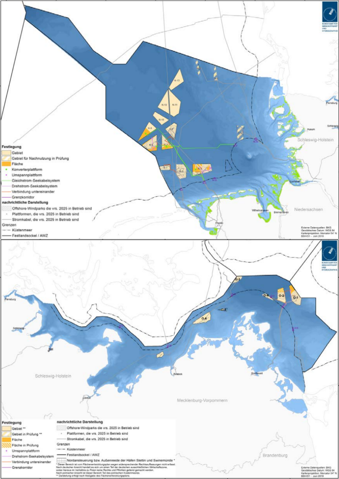
Areas for offshore wind park in North and Baltic sea. Source: NEP
PV ground mounted
The distribution of PV ground mounted is implemented in function insert
which is part of the dataset PowerPlants.
The following steps are conducted:
The sites and capacities of exisitng PV parks are imported using MaStR data (see Marktstammdatenregister).
Potential areas for PV ground mounted are assumed to be areas next to highways and railways as well as on agricultural land with a low degree of utilisation, as it can be seen in figure Example: sites of existing PV ground mounted parks and potential areas. Those areas (provided through the data bundle, see Data bundle) are imported while merging or disgarding small areas.
The locations of existing parks and the potential areas are intersected with each other while considering a buffer around the locations of existing parks to find out where there already are parks at or close to potential areas. This results in a selection of potential areas.
The capacities of the existing parks are considered and compared to the target values for the specific scenario per federal state (see Modeling concept and scenarios). The required expansion capacity is derived.
If expansion of PV ground mounted capacity is required, capacities are calculated depending on the area size of the formerly selected potential areas. The resulting parks are therefore located on the selected potential areas.
The resulting capacities are compared to the target values for the specific scenario per federal state. If the target value is exceeded, a linear downscaling is conducted. If the target value is not reached yet, the remaining capacity is distributed linearly among the rest of the potential areas within the state.
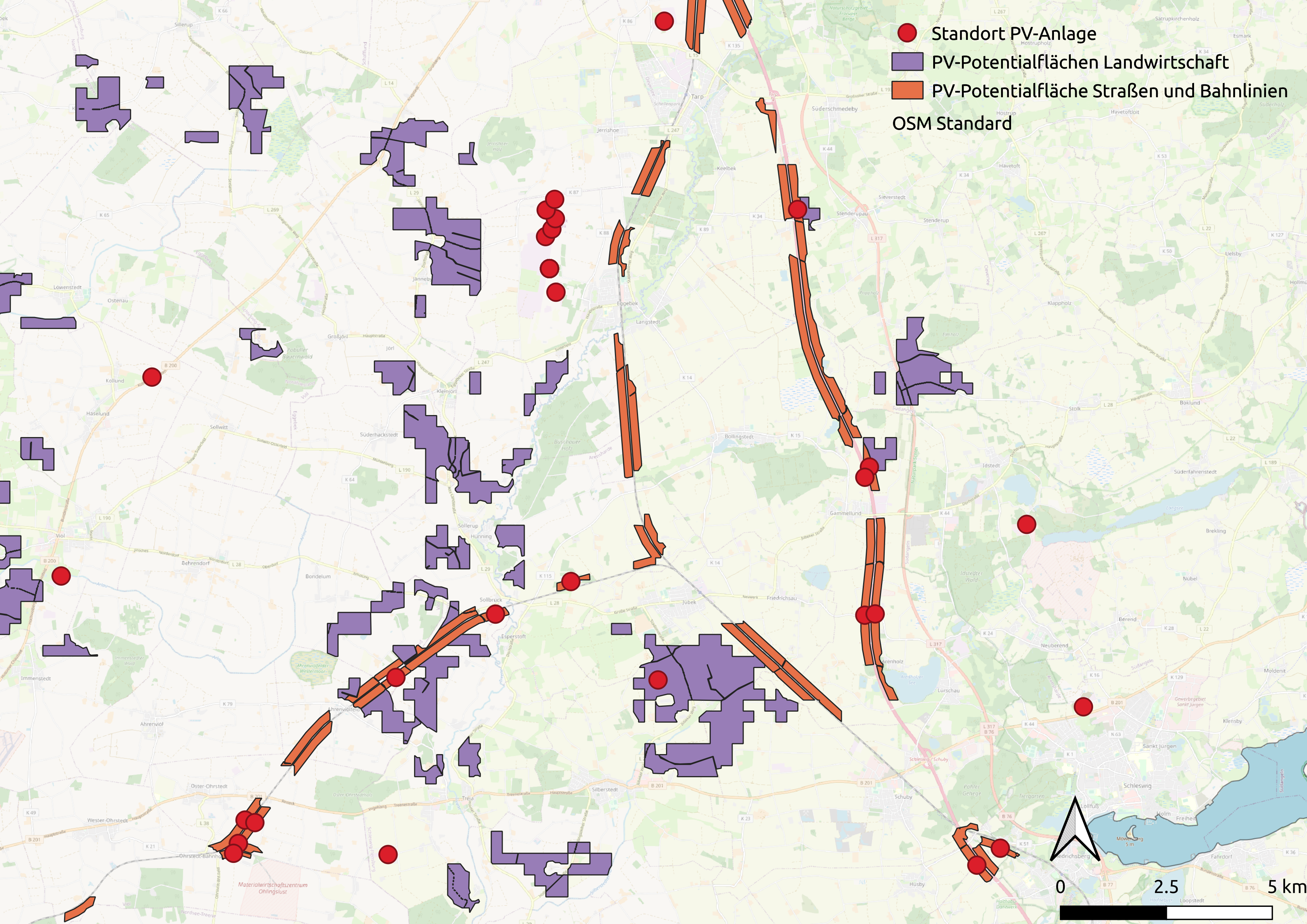
Example: sites of existing PV ground mounted parks and potential areas
PV rooftop
In a first step, the target capacity in the eGon2035 and eGon100RE scenarios is distributed
to all MV grid districts linear to the residential and CTS electricity demands in the
grid district (done in function
pv_rooftop_per_mv_grid).
Afterwards, the PV rooftop capacity per MV grid district is disaggregated
to individual buildings inside the grid district (done in function
pv_rooftop_to_buildings).
The basis for this is data from the MaStR, which is first cleaned and missing information
inferred, and then allocated to specific buildings. New PV plants are in a last step
added based on the capacity distribution from MaStR.
These steps are in more detail described in the following.
MaStR data cleaning and inference:
Drop duplicates and entries with missing critical data.
Determine most plausible capacity from multiple values given in MaStR data.
Drop generators that don’t have a plausible capacity (23.5 MW > P > 0.1 kW).
Randomly and weighted add a start-up date if it is missing.
Extract zip and municipality from ‘site’ given in MaStR data.
Geocode unique zip and municipality combinations with Nominatim (1 sec delay). Drop generators for which geocoding failed or which are located outside the municipalities of Germany.
Add some visual sanity checks for cleaned data.
Allocation of MaStR plants to buildings:
Allocate each generator to an existing building from OSM or a synthetic building (see Building data).
Determine the quantile each generator and building is in depending on the capacity of the generator and the area of the polygon of the building.
Randomly distribute generators within each municipality preferably within the same building area quantile as the generators are capacity wise.
If not enough buildings exist within a municipality and quantile additional buildings from other quantiles are chosen randomly.
Disaggregation of PV rooftop scenario capacities:
The scenario data per federal state is linearly distributed to the MV grid districts according to the PV rooftop potential per MV grid district.
The rooftop potential is estimated from the building area given from the OSM buildings.
Grid districts, which are located in several federal states, are allocated PV capacity according to their respective roof potential in the individual federal states.
The disaggregation of PV plants within a grid district respects existing plants from MaStR, which did not reach their end of life.
New PV plants are randomly and weighted generated using the capacity distribution of PV rooftop plants from MaStR.
Plant metadata (e.g. plant orientation) is also added randomly and weighted using MaStR data as basis.
Hydro
In the case of hydropower plants, a distinction is made between the carrier run-of-river
and reservoir.
The methods to distribute and allocate are the same for both carriers.
In a first step all suitable power plants (correct carrier, valid geolocation, information
about federal state) are selected and their installed capacity is scaled to meet the target
values for the respective federal state and scenario.
Information about the voltage level the power plants are connected to is obtained. In case
no information is availabe the voltage level is identified using threshold values for the
installed capacity (see assign_voltage_level).
In a next step the correct grid connection point is identified based on the voltage level
and geolocation of the power plants (see assign_bus_id)
The resulting list of power plants it added to table
EgonPowerPlants.
Biomass
The allocation of biomass-based power plants follows the same method as the one for hydro
power plants and is performed in function insert_biomass_plants
Conventional
CHP
non-chp
In function allocate_conventional_non_chp_power_plants
capacities for conventional power plants, which are no chp plants, with carrier oil and
gas are allocated.
Gas turbines
The gas turbines, or open cycle gas turbines (OCGTs) allow the production of electricity from methane and are modelled with unidirectional PyPSA links, which connect methane buses to power buses.
The capacities of the gas turbines are invariable and considered as constant. The technical parameters (investment and marginal costs, efficiency, lifetime) comes from the PyPSA technology data [technoData].
In Germany
In Germany, the gas turbines listed in the Netzentwicklungsplan [NEP2021]
are matched to the Marktstammdatenregister in order to get their geographical
coordinates in allocate_conventional_non_chp_power_plants.
The matched units are then associated to the corresponding power and methane
buses.
The implementation of gas turbines in the data model is detailed in the
OpenCycleGasTurbineEtrago
page of our documentation.
Warning
OCGT in Germany are still missing in eGon100RE: https://github.com/openego/eGon-data/issues/983
In the neighboring countries
In the scenario eGon2035, the gas turbines capacities abroad comes from the
TYNDP 2035 [TYNDP], the implementation is detailed in eGon2035.tyndp_gas_generation.
In the scenario eGon100RE the gas turbines capacities in the neighboring countries are taken directly from the PyPSA-eur-sec run.
Fuel cells
The fuel cells allow the production of electricity from hydrogen and are modelled with unidirectional PyPSA links, which connect hydrogen buses to power buses.
The data model contains the potentials of this technology, whose capacities are optimized. The technical parameters (investment and marginal costs, efficiency, lifetime) comes from the PyPSA technology data [technoData].
In the eGon2035 scenario, fuel cells are modelled at every hydrogen bus in Germany, as well as in the eGon100RE scenario. In eGon100RE, this technology is also modelled in the neighboring countries. In Germany, the potentials are generally not limited, except when the connected buses are located more than 500m far from each other. In this particular case, the potential has an upper limit of 1 MW.
The implementation of fuel cells in the data model is detailed in the
power_to_h2
page of our documentation.