High and extra-high voltage grids
The model of the German extra-high (eHV) and high voltage (HV) grid is based
on data retrieved from OpenStreetMap (OSM) (status January 2021) [OSM] and additional
parameters for standard transmission lines from [Brakelmann2004]. To gather all
required information, such as line topology, voltage level, substation locations,
and electrical parameters, to create a calculable power system model, the *osmTGmod*
tool was used. The corresponding dataset
Osmtgmod executes osmTGmod
and writes the resulting data to the database.
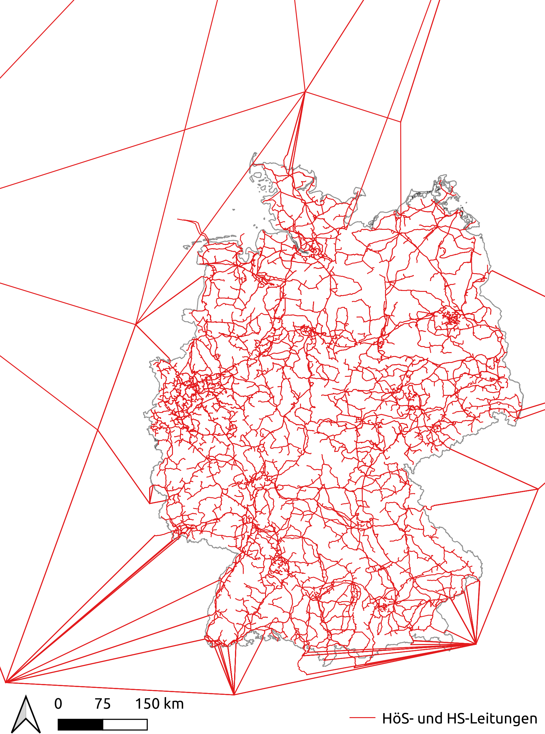
The resulting grid model includes the voltage levels 380, 220 and 110 kV and
all substations interconnecting the different grid levels. Information about
border crossing lines are as well extracted from OSM data by osmTGmod.
For further information on the generation of the grid topology please refer to [Mueller2018].
The neighbouring countries are included in the model in a significantly lower
spatial resolution with one or two nodes per country. The border crossing lines
extracted by osmTGmod are extended to representative nodes of the respective
country in dataset
ElectricalNeighbours. The
resulting grid topology is shown in the following figure.
Medium and low-voltage grids
Medium (MV) and low (LV) voltage grid topologies for entire Germany are generated using the python tool ding0 ding0. ding0 generates synthetic grid topologies based on high-resolution geodata and routing algorithms as well as typical network planning principles. The generation of the grid topologies is not part of eGon_data, but ding0 solely uses data generated with eGon_data, such as locations of HV/MV stations (see High and extra-high voltage grids), locations and peak demands of buildings in the grid (see Building data respectively Electricity), as well as locations of generators from MaStR (see Marktstammdatenregister). A full list of tables used in ding0 can be found in its config. An exemplary MV grid with one underlying LV grid is shown in figure Exemplary synthetic medium-voltage grid with underlying low-voltage grid generated with ding0. The grid data of all over 3.800 MV grids is published on zenodo.
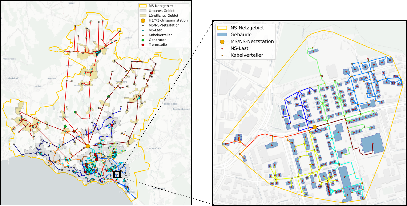
Exemplary synthetic medium-voltage grid with underlying low-voltage grid generated with ding0
Besides data on buildings and generators, ding0 requires data on the supplied areas by each grid. This is as well done in eGon_data and described in the following.
MV grid districts
Medium-voltage (MV) grid districts describe the area supplied by one MV grid. They are defined by one polygon that represents the supply area. Each MV grid district is connected to the HV grid via a single substation. An exemplary MV grid district is shown in figure Exemplary synthetic medium-voltage grid with underlying low-voltage grid generated with ding0 (orange line).
The MV grid districts are generated in the dataset
MvGridDistricts.
The methods used for identifying the MV grid districts are heavily inspired
by Hülk et al. (2017) [Huelk2017]
(section 2.3), but the implementation differs in detail.
The main difference is that direct adjacency is preferred over proximity.
For polygons of municipalities
without a substation inside, it is iteratively checked for direct adjacent
other polygons that have a substation inside. Speaking visually, a MV grid
district grows around a polygon with a substation inside.
The grid districts are identified using three data sources
Polygons of municipalities (
Vg250GemClean)Locations of HV-MV substations (
EgonHvmvSubstation)HV-MV substation voronoi polygons (
EgonHvmvSubstationVoronoi)
Fundamentally, it is assumed that grid districts (supply areas) often go along borders of administrative units, in particular along the borders of municipalities due to the concession levy. Furthermore, it is assumed that one grid district is supplied via a single substation and that locations of substations and grid districts are designed for aiming least lengths of grid line and cables.
With these assumptions, the three data sources from above are processed as follows:
Find the number of substations inside each municipality
Split municipalities with more than one substation inside
Cut polygons of municipalities with voronoi polygons of respective substations
Assign resulting municipality polygon fragments to nearest substation
Assign municipalities without a single substation to nearest substation in the neighborhood
Merge all municipality polygons and parts of municipality polygons to a single polygon grouped by the assigned substation
For finding the nearest substation, as already said, direct adjacency is preferred over closest distance. This means, the nearest substation does not necessarily have to be the closest substation in the sense of beeline distance. But it is the substation definitely located in a neighboring polygon. This prevents the algorithm to find solutions where a MV grid districts consists of multi-polygons with some space in between. Nevertheless, beeline distance still plays an important role, as the algorithm acts in two steps
Iteratively look for neighboring polygons until there are no further polygons
Find a polygon to assign to by minimum beeline distance
The second step is required in order to cover edge cases, such as islands.
For understanding how this is implemented into separate functions, please
see define_mv_grid_districts.
Load areas
Load areas (LAs) are defined as geographic clusters where electricity is consumed. They are used in ding0 to determine the extent and number of LV grids. Thus, within each LA there are one or multiple MV-LV substations, each supplying one LV grid. Exemplary load areas are shown in figure Exemplary synthetic medium-voltage grid with underlying low-voltage grid generated with ding0 (grey and orange areas).
The load areas are set up in the
LoadArea dataset.
The methods used for identifying the load areas are heavily inspired
by Hülk et al. (2017) [Huelk2017] (section 2.4).