The electricity demand considered includes demand from the residential, commercial and industrial sector. The target values for scenario eGon2035 are taken from the German grid development plan from 2021 [NEP2021], whereas the distribution on NUTS3-levels corresponds to the data from the research project DemandRegio [demandregio]. The following table lists the electricity demands per sector:
Sector |
Annual electricity demand in TWh |
|---|---|
residential |
115.1 |
commercial |
123.5 |
industrial |
259.5 |
A further spatial and temporal distribution of the electricity demand is needed for the subsequent grid optimization. Therefore different sector-specific distributions methods were developed and applied.
Residential electricity demand
The annual electricity demands of households on NUTS3-level from DemandRegio are scaled to meet the national target
values for the respective scenario in dataset DemandRegio.
A further spatial and temporal distribution of residential electricity demands is performed in
HouseholdElectricityDemand as described
in [Buettner2022].
The allocation of the chosen electricity profiles in each census cell to buildings
is conducted in the dataset
Demand_Building_Assignment.
For each cell, the profiles are randomly assigned to an OSM building within this cell.
If there are more profiles than buildings, all additional profiles are further randomly
allocated to buildings within the cell.
Therefore, multiple profiles can be assigned to one building, making it a
multi-household building.
In case there are no OSM buildings that profiles can be assigned to, synthetic buildings
are generated with a dimension of 5m x 5m.
The number of synthetically created buildings per census cell is determined using
the Germany-wide average of profiles per building (value is rounded up and only
census cells with buildings are considered).
The profile ID each building is assigned is written to data base table
demand.egon_household_electricity_profile_of_buildings.
Synthetically created buildings are written to data base table
openstreetmap.osm_buildings_synthetic.
The household electricity peak load per building is written to database table
demand.egon_building_electricity_peak_loads.
Drawbacks and limitations of the allocation to specific buildings
are discussed in the dataset docstring of
Demand_Building_Assignment.
The result is a consistent dataset across aggregation levels with an hourly resolution.
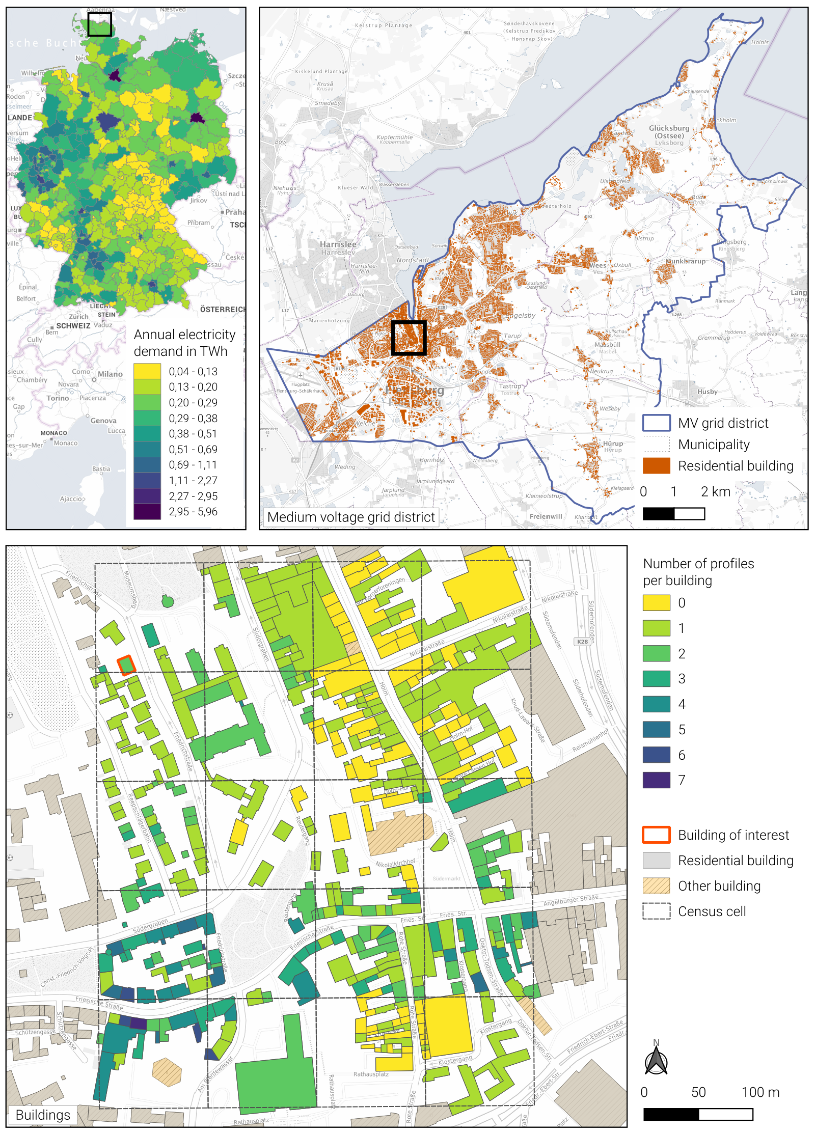
Electricity demand on NUTS 3-level (upper left); Exemplary MVGD (upper right); Study region in Flensburg (20 Census cells, bottom) from [Buettner2022]
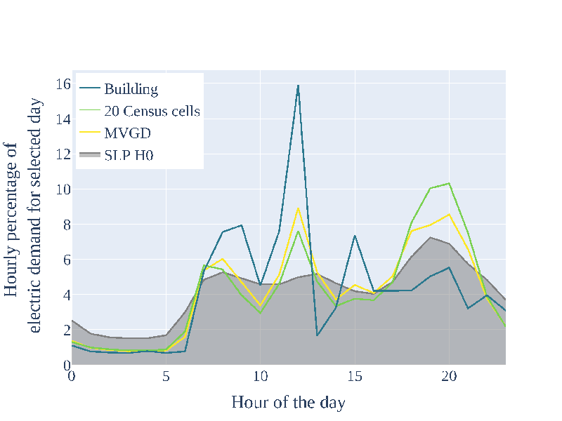
Electricity demand time series on different aggregation levels from [Buettner2022]
Commercial electricity demand
The distribution of electricity demand from the commercial, trade and service (CTS) sector is also based on data from
DemandRegio, which provides annual electricity demands on NUTS3-level for Germany. In dataset
CtsElectricityDemand the annual electricity
demands are further distributed to census cells (100x100m cells from [Census]) based on the distribution of heat demands,
which is taken from the Pan-European Thermal Atlas (PETA) version 5.0.1 [Peta]. For further information refer to section
Heat.
Spatial disaggregation of CTS demand to buildings
The spatial disaggregation of the annual CTS demand to buildings is conducted in the dataset
CtsDemandBuildings.
Both the electricity demand as well as the heat demand is disaggregated
in the dataset. Here, only the disaggregation of the electricity demand is described.
The disaggregation of the heat demand is analogous to it. More information on the resulting
tables is given in section Heat.
The workflow generally consists of three steps. First, the annual demand from Peta5 [Peta] is used to identify census cells with demand. Second, Openstreetmap [OSM] data on buildings and amenities is used to map the demand to single buildings. If no sufficient OSM data are available, new synthetic buildings and if necessary synthetic amenities are generated. Third, each building’s share of the HV-MV substation demand profile is determined based on the number of amenities within the building and the census cell(s) it is in.
The workflow is in more detail shown in figure Workflow for the disaggregation of the annual CTS demand to buildings and described in the following.
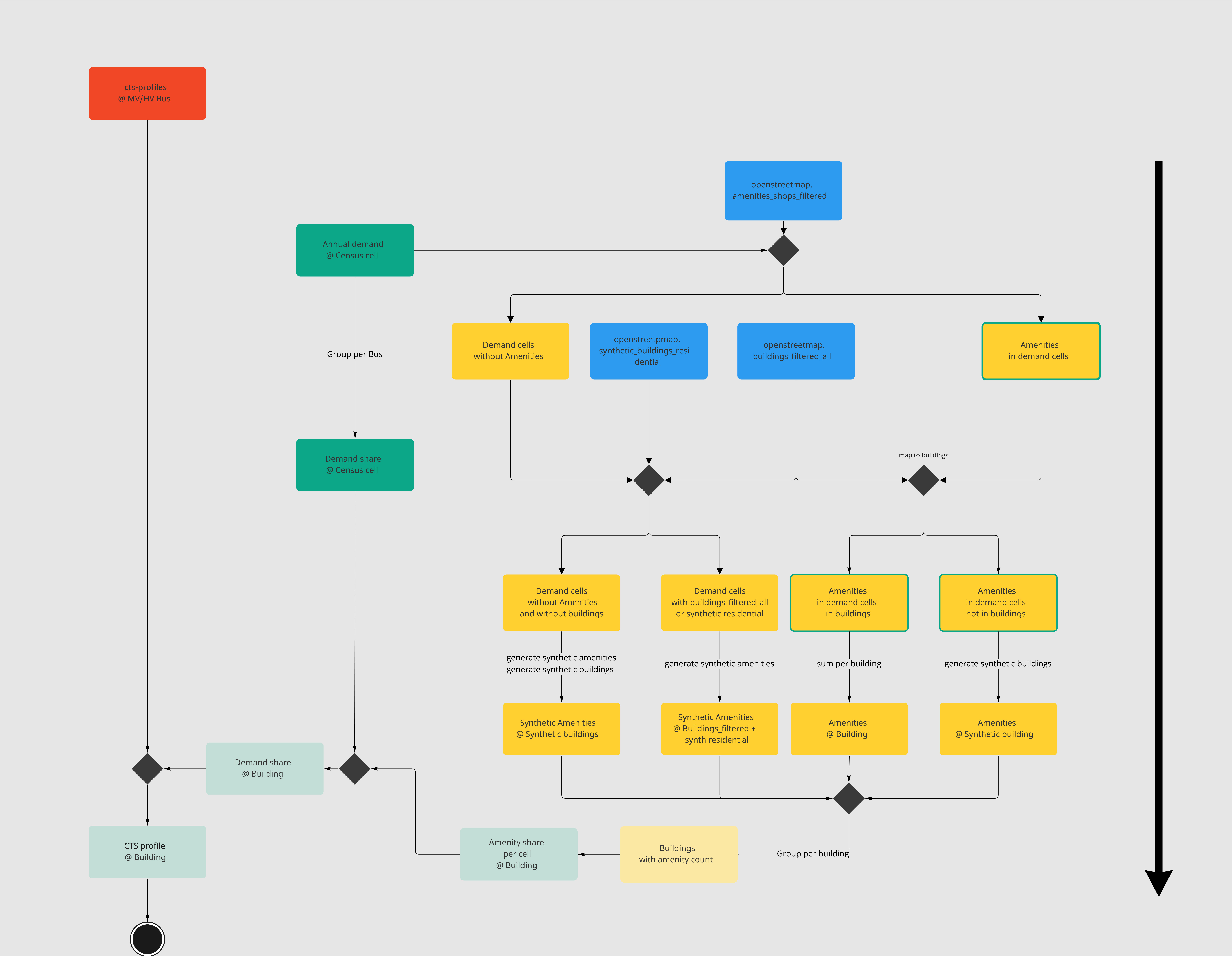
Workflow for the disaggregation of the annual CTS demand to buildings
In the OpenStreetMap dataset, we filtered all
OSM buildings and amenities for tags we relate to the CTS sector. Amenities are mapped
to intersecting buildings and then intersected with the annual demand at census cell level. We obtain
census cells with demand that have amenities within and census cells with demand that
don’t have amenities within.
If there is no data on amenities, synthetic ones are assigned to existing buildings. We use
the median value of amenities per census cell in the respective MV grid district
to determine the number of synthetic amenities.
If no building data is available, a synthetic building with a dimension of 5m x 5m is randomly generated.
This also happens for amenities that couldn’t be assigned to any OSM building.
We obtain four different categories of buildings with amenities:
Buildings with amenities
Synthetic buildings with amenities
Buildings with synthetic amenities
Synthetic buildings with synthetic amenities
Synthetically created buildings are written to data base table
openstreetmap.osm_buildings_synthetic.
Information on the number of amenities within each building with CTS, comprising OSM
buildings and synthetic buildings, is written to database table
openstreetmap.egon_cts_buildings.
To determine each building’s share of the HV-MV substation demand profile,
first, the share of each building on the demand per census cell is calculated
using the number of amenities per building.
Then, the share of each census cell on the demand per HV-MV substation is determined
using the annual demand defined by Peta5.
Both shares are finally multiplied and summed per building ID to determine each
building’s share of the HV-MV substation demand profile. The summing per building ID is
necessary, as buildings can lie in multiple census cells and are therefore assigned
a share in each of these census cells.
The share of each CTS building on the CTS electricity demand profile per HV-MV substation
in each scenario is saved to the database table
demand.egon_cts_electricity_demand_building_share.
The CTS electricity peak load per building is written to database table
demand.egon_building_electricity_peak_loads.
Drawbacks and limitations as well as assumptions and challenges of the disaggregation
are discussed in the dataset docstring of
CtsDemandBuildings.
Industrial electricity demand
To distribute the annual industrial electricity demand OSM landuse data as well as information on industrial sites are
taken into account.
In a first step (CtsElectricityDemand)
different sources providing information about specific sites and further information on the industry sector in which
the respective industrial site operates are combined. Here, the three data sources [Hotmaps], [sEEnergies] and
[Schmidt2018] are aligned and joined.
Based on the resulting list of industrial sites in Germany and information on industrial landuse areas from OSM [OSM]
which where extracted and processed in OsmLanduse the annual demands
were distributed.
The spatial and temporal distribution is performed in
IndustrialDemandCurves.
For the spatial distribution of annual electricity demands from DemandRegio [demandregio] which are available on
NUTS3-level are in a first step evenly split 50/50 between industrial sites and OSM-polygons tagged as industrial areas.
Per NUTS-3 area the respective shares are then distributed linearily based on the area of the corresponding landuse polygons
and evenly to the identified industrial sites.
In a next step the temporal disaggregation of the annual demands is carried out taking information about the industrial
sectors and sector-specific standard load profiles from [demandregio] into account.
Based on the resulting time series and their peak loads the corresponding grid level and grid connections point is
identified.
Electricity demand in neighbouring countries
The neighbouring countries considered in the model are represented in a lower spatial resolution of one or two buses per
country. The national demand timeseries in an hourly resolution of the respective countries is taken from the Ten-Year
Network Development Plan, Version 2020 [TYNDP]. In case no data for the target year is available the data is is
interpolated linearly.
Refer to the corresponding dataset for detailed information:
ElectricalNeighbours.